
Fundamentals of Fluid Flow in Porous Media
Chapter 5
Miscible Displacement
Fluid Properties in Miscible Displacement: Macroscopic Displacement Efficiency
Mixing of Fluid by Dispersion
In all miscible displacement processes mixing occurs between the displacing and displaced fluids. That is there is dispersion between the different fluids. This dispersion dilutes the displacing fluid with the displaced fluid and thereby affects the phase behavior.
Suppose a first contact miscible solvent is injected into a linear tube to displace an oil that has the same density and viscosity as the solvent. Viscosity and density difference has no effect on the displacement and flow behavior. Concentration of the solvent at the outlet face of the tube is measured with time to find a concentration profile of the solvent versus time. Figure 5‑46 shows two different concentration profile of the solvent in effluent versus time. Figure 5‑46.a is the concentration that we expected according to mobility ratio equal to one and no gravity effect. We expect to see the solvent in the effluent after injection of one pore volume (equal to the tube volume, here) of solvent and the concentration is expected to reach its maximum value immediately (Figure 5‑46.a) . But Figure 5‑46.b is the concentration profile that we get in the real word. Solvent in the effluent is detected before injection of one pore volume. S-shaped concentration profile resulted from mixing, or dispersion of solvent and oil in the tube. At first, solvent is produced at low concentration. This is followed by a period of sleepy rising concentration and finally by a period where effluent concentration gradually approaches injected concentration. The same phenomenon happens in porous media. During the solvent injection into a linear tube packed with sand there is a transition zone between pure solvent/oil because of mixing. The S-shaped curve in Figure 5‑46.b is the classic concentration for miscible displacement of one fluid with a second in a linear system in which the mobility ratio is favorable and gravity effect is negligible.
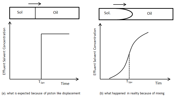
Figure 5-46: Profile of the Solvent Effluent Concentration Produced from a Capillary Tube in an Equal Viscosity and Density
As another illustration consider the injection of a small slug of fluid B into packed tube saturated with fluid A. small slug of B in followed by injection of A. the concentration profile at the inlet at the first time would be like as Figure 5‑47. If the concentration of solvent is measured at different position of the capillary tube at a fixed time after injection Figure 5‑47.a is what is expected in the absence of mixing, or dispersion. But in real condition the concentration profiles would tend to spreads as the fluid moved downstream, and the amplitude (maximum concentration) would decrease (Figure 5‑47.b).
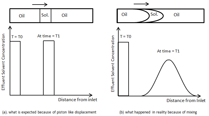
Figure 5-47: Concentration Profile for Injection of a Slug of Solvent to Displace Oil
This mixing in the direction of primary flow is called “Longitudinal Dispersion”. Dispersion also occurs in transvers direction – that is in a direction perpendicular to flow:
Assume solvent injection to a two dimensional model. The model contains two layer of sand. One of the layers is much more permeable than the other such that solvent, which is injected across the left face of the model, mostly enters only the permeable layer. The solvent and oil have the same viscosity and density. In this experiment, the solvent not only mixes with the oil by longitudinal dispersion in the direction of flow; it also mixes with oil transverse to the direction of flow in the less permeable (Figure 5‑48). If concentration were measured in situ through the section marked AA, an S-shaped concentration profile again would be found. This mixing transverse to the direction of flow is called “Transverse Dispersion”.
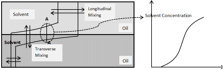
Figure 5-48: Mixing of Solvent and Oil by Longitudinal and Transverse Dispersion
The dispersion of miscible fluids may be attributed to several phenomena:
Molecular Diffusion: is present in all systems in which miscible fluids are bought into physical contact. The diffusion process is molecular in nature; i.e., it results from the random motion of molecules in solution. Diffusion is dominated dispersion mechanism if flow rates are very low in a porous medium. At rates that commonly exist in reservoir displacement processes, however, dispersion also results from bulk flow or convection phenomenon.
Velocity profile (Taylor) effect: Taylor showed that dispersion that occurs during the miscible displacement process in a straight capillary tube (Figure 5‑46.b), is a result of velocity profile in the capillary tube. Assume that fluid A is initially in the capillary and that the fluid B displaces fluid A. assume further that the flow rate is low so that flow is laminar. The velocity profile radially across the capillary tube would have the parabolic form (Figure 5‑46.b). the profile would be such that:

And the maximum velocity occurs at the center of tube. If the effluent from the capillary were collected and the concentration measured, breakthrough of fluid B would occur when a volume equal to one-half of the capillary volume had been injected. With continued injection concentration of B increase till there was no more fluid A in the effluent. Thus mixing occurs because of the velocity profile that develops in laminar flow in a capillary. Molecular diffusion also occurs across the fluid A/B boundaries in the capillary.
Series of mixing cells: another model for the mixing of miscible fluids is based on the assumption that a porous medium is a series of mixing cells or tanks in which fluids perfectly mixed. () illustrate this concept. Fluid B (solvent) enters a pore (Tank1) from the left. Fluids in the tank are perfectly mixed; i.e. there is no concentration gradient in the tank. This assumption means that at any instance there is no concentration difference between the effluent fluid concentration of the tank and fluid in the tank. The mixed fluid from the first pore enters to the next pore, where the fluids are again perfectly mixed. So such model will lead to dispersion of fluid B into fluid A as the displacement process continuous.
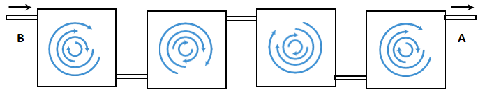
Figure 5-49: Dispersion Porous Medium Being Viewed as a Series of Mixing Tank
Stagnant pockets: another contribution to dispersion can be attributed to the flow behavior around stagnant pockets or dead end pores. Assume fluid B displaces fluid A. the part of fluid A that is in the main flow channel is displaced directly by fluid B. however some part of fluid A are in in stagnant pockets or dead end pores- i.e., pore spaces that are connected to the main channels but through which there is no flow. This quantity of fluid A is not displaces directly but is initially bypassed by fluid B. displacement of this bypassed fluid does occur slowly as a result of molecular diffusion between the main flow channel and the stagnant pocket. The overall result of this process is to cause mixing of fluid A and B in the medium as the displacement progresses through the system. The consequence of finite-rate mass transfer between the flowing and stagnant fractions is an increase in the length of the mixing zone. The trapping of fluid in dead-end pores is termed “capacitance.” Some simple configurations of stagnant volume that have been used to model capacitance are shown in Figure 5‑50.
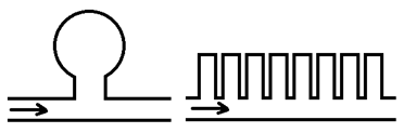
Figure 5-50: Stagnant Volume Models
The effect of the capacitance could be distinguished in effluent concentration profile. In the absence of the capacitance (stagnant volume), effluent concentration profile has a symmetric s-shaped as shown in (Figure 5‑50). In the presence of stagnant pockets tracer effluent profiles from porous media are characterized by tailing or deviation from the symmetrical S-shape (Figure 5‑51).
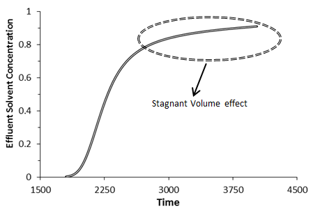
Figure 5-51: The Effects of Capacitance
Variation in flow path: dispersion of fluid B into fluid A can result from the variation of flow paths through the media encountered by different fluid particles. As before, fluid A is being displaced by fluid B. visualize two separate particles (very small quantities) of fluid B located at point 1 in Figure 5‑51. As flow progresses, the particles moves downstream to point 2 but by slightly different paths through the medium. Because the flow paths are different, the particles arrive downstream at different time. That is, dispersion of the fluid has resulted directly from the tortuosity inherent in the porous medium. Fluids become mixed because flow paths are varied as flow progresses through the system.
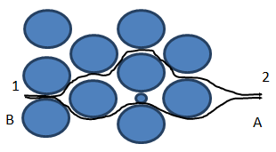
Figure 5-52: Dispersion Caused by Variation of Flow Paths in a Porous Medium
[fusion_builder_container hundred_percent=”yes” overflow=”visible” margin_top=”25″ margin_bottom=”” background_color=”rgba(255,255,255,0)”][fusion_builder_row][fusion_builder_column type=”1_1″ background_position=”left top” background_color=”” border_size=”” border_color=”” border_style=”solid” spacing=”yes” background_image=”” background_repeat=”no-repeat” padding=”” margin_top=”0px” margin_bottom=”0px” class=”” id=”” animation_type=”” animation_speed=”0.3″ animation_direction=”left” hide_on_mobile=”no” center_content=”no” min_height=”none”][fusion_separator /]
[/fusion_builder_column][/fusion_builder_row][/fusion_builder_container][fusion_builder_container hundred_percent=”yes” overflow=”visible”][fusion_builder_row][fusion_builder_column type=”1_2″ last=”no”]
<< OPTIMIZATION OF VERTICAL MISCIBLE FLOOD PERFORMANCE THROUGH CYCLIC PRESSURE PULSING
[/fusion_builder_column]
[fusion_builder_column type=”1_2″ last=”yes”]
[/fusion_builder_column]
[fusion_builder_column type=”1_1″ background_position=”left top” background_color=”” border_size=”” border_color=”” border_style=”solid” spacing=”yes” background_image=”” background_repeat=”no-repeat” padding=”” margin_top=”0px” margin_bottom=”0px” class=”” id=”” animation_type=”” animation_speed=”0.3″ animation_direction=”left” hide_on_mobile=”no” center_content=”no” min_height=”none”][fusion_separator top=”35″/]
References
[/fusion_builder_column][fusion_builder_column type=”1_1″ background_position=”left top” background_color=”” border_size=”” border_color=”” border_style=”solid” spacing=”yes” background_image=”” background_repeat=”no-repeat” padding=”” margin_top=”0px” margin_bottom=”0px” class=”” id=”” animation_type=”” animation_speed=”0.3″ animation_direction=”left” hide_on_mobile=”no” center_content=”no” min_height=”none”][1]
Questions?
If you have any questions at all, please feel free to ask PERM! We are here to help the community.[/fusion_builder_column][/fusion_builder_row][/fusion_builder_container]