
Fundamentals of Fluid Flow in Porous Media
Chapter 5
Miscible Displacement
The Equation of Continuity in Porous Media: Solutions to the One-Dimensional Convection-Dispersion Model
Infinite System
For a single solute and no source/sink, Eq. (5‑56) becomes:

The following assumptions are implicit in eq. (5‑68):
- homogeneous porous medium of constant cross-section;
- bulk flow in the axial direction at constant interstitial velocity;
- constant fluid density;
- constant dispersion coefficient;
- incompressible porous medium;
- uniform concentration distribution in the direction perpendicular to flow (i.e., time is “long” enough for the convection-dispersion model to hold);
- no solute sources or sinks.
Eq. (5‑68) is a second order partial differential equation, requiring two boundary and an initial condition for its solution.
When the space variable x is translated such that the transformed distance x’ becomes the distance from the flood front rather than the distance from the inlet of the porous medium, eq. (5‑68) reduces to the one-dimensional unsteady diffusion or heat conduction equation, also known as Fick’s second law (Taylor, 1953; Nunge and Gill, 1970):

Where,
x’ = x – vt
And,
vt = distance of the flood front from the porous medium entrance.
This equation has been solved analytically for a variety of initial and boundary conditions (see, for example, Carslaw and Jaeger, 1959; Özişik, 1980).
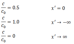
Consider an infinite porous medium at zero initial concentration, with a step change in inlet concentration (c0):
| t = 0 | x’ ≥ 0 | c = 0 | (5‑70) |
| x’ < 0 | c = c0 | ||
| t > 0 | x’ → -∞ | c → c0 | |
| x’ → +∞ | c → 0 |
The solution to eq. (5‑69) with initial and boundary conditions (5‑70) is (Danckwerts, 1953; Brigham et al., 1961):

Where,
c / co = normalized concentration,
er ƒ(r) = error function of a variable r:

Some properties of the error function are
[fusion_builder_container hundred_percent=”yes” overflow=”visible”][fusion_builder_row][fusion_builder_column type=”1_3″ last=”no”]
er ƒ(0) = 0
[/fusion_builder_column]
[fusion_builder_column type=”1_3″ last=”no”]
er ƒ(∞) = 1
[/fusion_builder_column]
[fusion_builder_column type=”1_3″ last=”yes”]
er ƒ(-r) = er ƒ(r)
[/fusion_builder_column]
Then, from eq. (5‑71),
Typical concentration profiles, obtained from Equation 23, are shown in Figure 6. The curves are symmetrical about the point ( z’ = 0, c / c0 = 1/2). The profiles become more dispersed when D increases or as time progresses.
In non-dimensional form, eq. (5‑68) becomes:

Where,
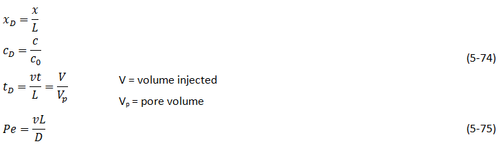
Initial and boundary conditions can similarly be put into non-dimensional form.
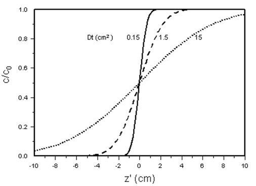
Figure 5-58: Concentration as a Function of Transformed Distance for Different Values of Dispersion Coefficient or Time, Calculated from eq. (5-72), Infinite System
The convection-dispersion model thus contains a single parameter: the dispersion coefficient, or, in dimensionless form, the Peclet number. The Peclet number represents the ratio of characteristic times for mass transfer by flow and by dispersion, and is a measure of the length of the mixing zone relative to the length of the porous medium. The Peclet number, as defined in eq.5‑75), contains the porous medium length as characteristic length, because L is a parameter easily measured in laboratory experiments. Other characteristic lengths have been used in the definition of the Peclet number, as is evident from the discussions above. Also, depending on the process under investigation, the denominator may contain the diffusion coefficient or the dispersion coefficient. Regions of flow where different models apply in any given system are often characterized in terms of the Peclet number, as, for example, in Figure 5‑56.
[fusion_builder_column type=”1_1″ background_position=”left top” background_color=”” border_size=”” border_color=”” border_style=”solid” spacing=”yes” background_image=”” background_repeat=”no-repeat” padding=”” margin_top=”0px” margin_bottom=”0px” class=”” id=”” animation_type=”” animation_speed=”0.3″ animation_direction=”left” hide_on_mobile=”no” center_content=”no” min_height=”none”][fusion_separator top=”25″/]
[/fusion_builder_column][fusion_builder_column type=”1_2″ last=”no”]
<< EQUATION OF DISPERSION IN POROUS MEDIA
[/fusion_builder_column]
[fusion_builder_column type=”1_2″ last=”yes”]
DETERMINATION OF THE DISPERSION COEFFICIENT >>
[/fusion_builder_column]
[fusion_builder_column type=”1_1″ background_position=”left top” background_color=”” border_size=”” border_color=”” border_style=”solid” spacing=”yes” background_image=”” background_repeat=”no-repeat” padding=”” margin_top=”0px” margin_bottom=”0px” class=”” id=”” animation_type=”” animation_speed=”0.3″ animation_direction=”left” hide_on_mobile=”no” center_content=”no” min_height=”none”][fusion_separator top=”35″/]
References
[/fusion_builder_column][fusion_builder_column type=”1_1″ background_position=”left top” background_color=”” border_size=”” border_color=”” border_style=”solid” spacing=”yes” background_image=”” background_repeat=”no-repeat” padding=”” margin_top=”0px” margin_bottom=”0px” class=”” id=”” animation_type=”” animation_speed=”0.3″ animation_direction=”left” hide_on_mobile=”no” center_content=”no” min_height=”none”][1]
Questions?
If you have any questions at all, please feel free to ask PERM! We are here to help the community.[/fusion_builder_column][/fusion_builder_row][/fusion_builder_container]