[1]
One important example of interface encroachment is the local deformation of the interface (G/O or O/W) near a producing well.  Draw off caused by a pressure difference between the well and the interface caused the interface to be distorted and to approach the well.  If the well is in production and the medium is homogeneous and isotropic, then the flow follows symmetry of revolution.  However, if the flow is not exactly radial-cylindrical and the well is not perforated along the entire thickness of the bed, then the stream lines in the lower portion of the bed straighten upwards to reach the base of the well (O/W interface).  This upward flow of the oil and water distorts the water/oil contact surface, which then assumes a roughly conical shape.  Several types of coning can occur according to the input and distribution conditions of the fluids.  Figure 4‑24 illustrates the two main types: bottom coning and edge coning.

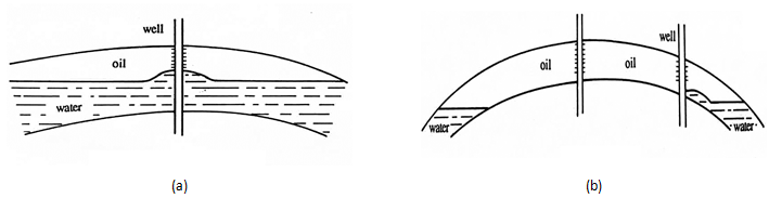
Figure 4-24: a) Bottom Coning at Oil-Water or Gas-Oil Contact, b) Edge Coning at Oil-Water or Gas-Oil Contact

Figure 4‑25 shows a borehole that has been drilled to depth, hp, in a layer of thickness, H.  This layer is impregnated with oil to height, h_o, and by water to height ( H – h_o ).  The ratio h_p / h_o is the penetration of the borehole.  The greater the draw off effect of the well, i.e. the greater the penetration and flow rate, the higher the “cone”.  Conversely, gravitational forces exert a stabilizing effect.

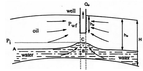
Figure 4-25: Stable Cone

Infra-Critical Flow

For a set of given values of the parameters shown in Figure 4‑25, and if the flow rate is sufficiently low with respect to penetration, the cone will form a fixed surface in space.  Such a cone is stable and does not reach the base of the perforations.  Also, no water encroachment occurs in the well shown in Figure 4‑25.  Note that at critical flow a further increase in pressure differential will not increase the flow rate.

Supercritical Flow

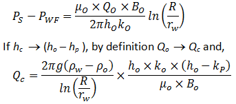
This section includes only a discussion of bottom coning as edge coning requires very complex analysis and is studied by simulation.  Investigations conducted by Bournazel and Jeanson (IFP) clarify the correlations established by Sobocinsky (Esso) concerning bottom coning.  The critical flow rate is given by the following equation, in US field units (barrels per day, pounds per cubic foot, millidarcys, feet, centipoise):

Where,

∝ = 1.41×10^-5 (Sobocinsky) and

∝ = 1.15×10^-5 (Bournazel and Jeanson correlation results).

If metric units are used, ∝ = 1.52×10^-3 and ∝ = 1.24×10^-3, respectively.

This formula is derived from the expression of the forces in Figure 4‑25:

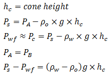
Using Darcy’s Law:

With,

h_o – h_p = water blanket

The coefficient ∝ is obtained from an average correlation including ln( R / r_w ) and the partial penetration effect.  It is important to note that the critical flow rate is dependent on the horizontal permeability k_h.  Additionally, the well results often give a critical flow rate higher than the one given by this equation.  This is partly a result of the assumption that the formation of the cone is considered “statically” whereas the vertical movement of water also occurs, and partly because little is known about the permeabilities, k_h and k_v, near the well.

Bournazel’s study also provided a methodology to calculate the breakthrough time and the change in the WOR after breakthrough, and that the WOR reaches a limit for horizontal input and steady-state flow.

Although coning has been investigated methodically since the 1950’s, it is so complex and unstable that two basic questions remain unanswered:

1. How to drill a well subject to coning?
2. What is the correct production rate?

Controversies exist on these subjects.  The cautious solution involves perforating over a short stretch of pay zone and adopting a low flow rate to delay the arrival of the undesirable fluid at the well for as long as possible.  This method is adopted if Q_o it is not much higher than Q_c, see (1) in Figure 4‑26.

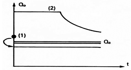
Figure 4-26: Flow Rate versus Time

From this standpoint, it would be better to avoid drilling a well crossing the O/W, G/O or G/W interfaces with a large thickness of undesirable fluid.

However, the more recent “full pot” solution involves perforating widely and withdrawing at maximum flow rate (see (2) in Figure 4‑26), with considerable production of the second fluid, if the second fluid is mostly comprised of water.  In fact, at largely supercritical conditions, the final recovery can be improved with high flow rates.

It should be added that empirical laws serve to make production forecasts for coning in supercritical conditions after breakthrough.  Included are the methods of Hutchinson and Henley, who established correlations between recovery and WOR as a function of the mobility ratio, the estimated recovery area and the penetration or the flow rate.

However, numerical models adapted for coning are widely employed to simulate these problems.  A vertical subdivision is used to represent the horizontal and vertical permeability variations of the reservoir, providing a better approximation of the potential results.  Also, various assumptions regarding heterogeneities serve to achieve some sensitivity in the results.

Studies are also under way to prevent water influxes by injecting polymers that are designed to plug the water influx zones.

References

[1] Cossé, R., Houston: Gulf Publishing Company, 1993.

Questions?

If you have any questions at all, please feel free to ask PERM!  We are here to help the community.