Fundamentals of Fluid Flow in Porous Media

 

Chapter 5

Miscible Displacement

The Equation of Continuity in Porous Media: Solutions to the One-Dimensional Convection-Dispersion Model

Determination of the Dispersion Coefficient

Because of its simplicity, eq. (5‑71), although representing infinite systems, is often used to approximate concentration distributions in finite systems. In a typical laboratory core flood experiment, a porous medium is fully saturated with a fluid. A miscible fluid or tracer, such as a salt solution or dye or radioactive material, is then injected at a known, constant flow rate. Effluent samples are collected at the core exit and analyzed for tracer concentration. In such an experiment, eq. (5‑71) represents the effluent concentration, i.e., the concentration at a fixed distance ( z = L, or z’ = L – vt ).

In an experiment such as this one, the dispersion coefficient can be determined using a simple procedure described by Brigham et al. (1961). When eq. (5‑71) is used to calculate effluent concentrations from a finite porous medium ( z = L or z’ = L – vt ), it is convenient to transform variables such that time is replaced by throughput in pore volumes (Brigham et al., 1961; Brigham, 1974). Change variables such that:

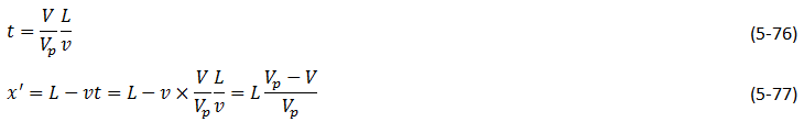
Eq. (5‑71) then becomes:

Where,

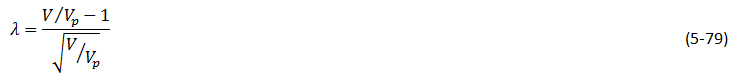
When λ is plotted against the percentage of displacing fluid in the effluent on arithmetic probability coordinates (Figure 5‑59), and provided the convection-dispersion model holds, a straight line results from which the longitudinal dispersion coefficient can be obtained using the following equation (Brigham et al., 1961; Perkins and Johnston, 1963):

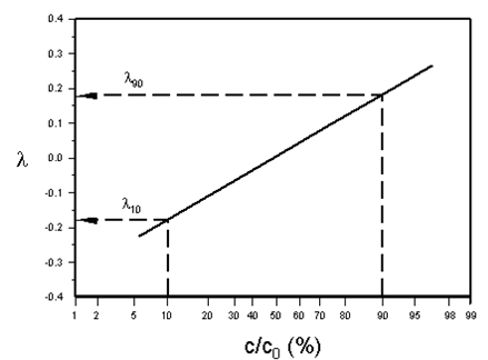
Figure 5-59: Typical Probability Plot for Determination of Longitudinal Dispersion Coefficient

λ₁₀ and λ₉₀ are the values of λ when the effluent concentration is 10% and 90% of the injected value, respectively, and v and L are known experimental parameters. The constant 3.625 arises from the error function and the choice of 10% and 90% concentrations. When 20% and 80%, or 5% and 95%, concentrations are used instead, this constant becomes 2.380 or 4.653, respectively.

Alternatively, the dispersion coefficient can be determined by plotting experimental effluent concentration profiles against volume injected and adjusting D until Equation 30 fits the experimental data. This is commonly done with effluent concentrations, since they are easily measured through chemical analysis. In-situ concentrations may also be used, but generally require more sophisticated experimental methods, for example x-ray or nuclear magnetic resonance techniques. In-situ concentrations can be modeled as a function of time and distance using eq. (5‑71).

When experimental effluent concentrations are plotted on probability coordinates, it is assumed that they are described by the error function (eq. (5‑78)), i.e. that the porous medium can be approximated by an infinite system. Analytical solutions to eq. (5‑68) for semi-infinite or finite systems contain an error function in addition to other terms. Theoretically, they should not result in a linear probability plot, particularly at low Peclet numbers (Pe < 30). However, in practice it has been found that a probability plot is often linear for finite systems and, in addition, yields the correct dispersion coefficient even at Peclet numbers as low as 14 (Brigham, 1974). Shuler (1978) found that dispersion coefficients determined by fitting a finite system convection-dispersion model to tracer data were very similar to coefficients obtained from probability plots for the range of Peclet numbers investigated (Pe between 140 and 420). The probability plot is therefore commonly used to determine dispersion coefficients for systems other than infinite. In fact, a probability plot is often used to determine whether the convection-dispersion model is valid for a given set of experimental data (Brigham, 1974). Deviation of a probability plot from linearity indicates that a more complex model may be required to describe mass transport.

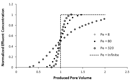
Figure 5-60: Effluent Concentration Profiles for a Range of Peclet Numbers, Calculated from eq. (5-78), Infinite System

Figure 5‑60 shows effluent concentrations plotted as a function of pore volumes injected (eq. (5‑78)). As in Figure 5‑58, the mixing zone becomes wider as the dispersion coefficient increases, or as Pe decreases. According to eq. (5‑78), c / c₀ = 1/2 at one pore volume injected. When D → 0 (Pe → ∞), plug flow is obtained and the effluent profile is a step function. When D → ∞ (Pe → 0), the porous medium becomes a continuous stirred tank, and the dispersion model no longer holds.

It is of interest to note that the curves in Figure 5‑58, which represent concentrations at a fixed value of time plotted as a function of distance, are always symmetrical. By contrast, the concentrations in Figure 5‑60, which are concentrations at a fixed distance ( z = L ) plotted as a function of time or throughput, are not symmetrical, particularly at low Peclet numbers. This may seem surprising, since both sets of curves are derived from solutions to the same equation. The reason for the difference in symmetry is evident from eqs. (5‑71) and (5‑78). At a fixed value of time, concentrations calculated from equation 23 are always symmetrical about the flood front ( z = vt or z’ = 0 ). Concentrations calculated as a function of time or pore volumes injected at z=L from eq. (5‑78) are not symmetrical about a throughput of one pore volume because of the term ( √(V / V_p) ) that appears in the denominator of the error function argument. The asymmetry becomes more pronounced at low Peclet numbers. Brigham (1974) has previously noted this, and has discussed the implications in detail.