Fundamentals of Fluid Flow in Porous Media

 

Chapter 5

Miscible Displacement

The Equation of Continuity in Porous Media: Solutions to the One-Dimensional Convection-Dispersion Model

Alternative Boundary Conditions

Alternative boundary conditions have been used to solve eq. (5‑68), specifying concentration (Dirichlet boundary condition), flux (Neumann boundary condition), or a combination of both (Robin’s boundary condition). The following initial and boundary conditions have been commonly used to represent finite and semi-infinite systems:

Where c_o can be a function of time, but is often taken as a constant, and c_a is the initial concentration in the porous medium and can be zero, or a constant, or a function of distance.

These boundary conditions have been discussed quite widely, for example by Danckwerts (1953), Kramers and Alberda (1953), Aris and Amundson (1957), Bischoff and Levenspiel (1962), Coats and Smith (1964), and Brigham (1974). Inlet condition 5‑83) states that the solute concentration at the entrance to the porous medium is determined by bulk flow and diffusion. Outlet condition 5‑86) is somewhat intuitive, and is necessary to prevent the solute concentration in a porous medium of finite length from passing through a maximum or minimum (Danckwerts, 1953). Conditions 5‑83) and 5‑86) are often referred to as “Danckwerts’ boundary conditions.” Outlet condition 5‑87) has been used by Batycky et al. (1982), who argue that it is less restrictive than the Danckwerts condition 5‑86), and is computationally more convenient to use than the semi-infinite bed condition.

Analytical solutions to eq. (5‑71) with different boundary conditions are readily available in the literature. References to some of these papers have been tabulated, with boundary conditions, by Mannhardt and Nasr-El-Din (1994), and include Danckwerts (1953), Gershon and Nir (1969), Bear (1972), Brighham (1974), Coats and Smith (1964), Fried and Combarnous (1971), Brenner (1962), Sorbie et al. (1985). Van Genuchten and co-workers have published extensive compilations of analytical solutions (Parker and van Genuchten, 1984; Toride et al., 1993; van Genuchten, 1981; van Genuchten and Alves, 1982).

Many solutions to the convection-dispersion equation for systems other than infinite contain the error function in addition to other terms, and c / c_o is therefore different from 0.5 at V / V_p = 1. Different concentration profiles are obtained when different boundary conditions are used to solve eq. (5‑61), particularly when the mixing zone is large compared to the length of the porous medium, i.e., when Pe is small (Brigham, 1974). An example of effluent profiles with boundary conditions 5‑83) and 5‑86), and zero initial concentration, is shown in Figure 5‑61 (Brenner, 1962). In the absence of dispersion ( Pe → ∞, D = 0 ), the effluent concentrations are a step function. As dispersion increases (Pe decreases), the effluent concentrations take the symmetrical S-shape often observed in experimental data. c / c₀ is greater than ½ at one pore volume injected at small Pe, but approaches ½ with increasing Pe. When Pe = 0 (D → ∞), the porous medium becomes a continuous stirred tank. The convection-dispersion model no longer applies, and the effluent concentrations become an exponential function of the volume injected.

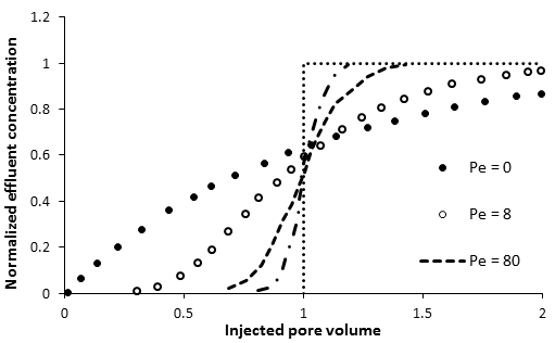
Figure 5-61: Effluent Concentration Profiles for a Range of Peclet Numbers, Finite System with Danckwerts’ Boundary Conditions (Brenner, 1962)

The solution to eq. (5‑71) is thus sensitive to the boundary conditions. Examples of effluent curves for an infinite system with a step change in input concentration (boundary conditions (5‑70)) and for a finite system with boundary conditions 5‑83) and 5‑86) are shown in Figure 5‑62. At a Peclet number of 24, differences in effluent concentrations from the two systems become quite small. A detailed comparison of solutions to the convection-dispersion model, obtained with different boundary conditions, is provided by Gershon and Nir (1969) and van Genuchten and Alves (1982). The latter authors suggest that differences between solutions become small compared to experimental errors when the Peclet number exceeds 30.

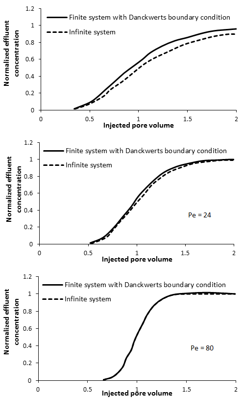
Figure 5-62: Effect of Boundary Conditions on Solutions to the Convection-Dispersion Equation at Different Peclet Numbers

The proper choice of inlet boundary condition in a semi-infinite system with outlet condition 5‑84), with c_a = 0, has been discussed by Brigham (1974), and later by Parker and van Genuchten (1984) and Toride et al. (1993), who argue that one must distinguish between “flowing” and “in-situ” concentrations, related through the following equation:

Where,

c’ = Flowing concentration,

c = In-situ concentration.

Eq. (5‑88) states that the concentration flowing from a differential volume element of porous medium is different from the in-situ concentration inside the volume element because mass transfer of solute is due to the combined effects of convection and dispersion. Depending on the concentration gradient, the flowing concentration can be larger or smaller than the in-situ concentration.

Eq. (5‑71) represents both flowing and in-situ concentrations. However, which concentration is represented by any specific solution to Eq. (5‑71) is determined by the boundary conditions. Boundary condition 5‑82) represents flowing concentration (the concentration being injected into the porous medium), and the solution to equation (5‑68) at z = L using this boundary condition thus represents effluent concentrations (“effluent” implying “flowing”). When the convection-dispersion model is applied to concentrations that are measured in-situ, boundary condition (5‑83), representing in-situ concentrations, should be used. No matter which concentrations are used, one can interconvert between in-situ and flowing concentrations using equation 40. Brigham (1974) concludes that it makes little difference which boundary conditions one uses, provided the solution to Equation (5‑68) is interpreted properly in terms of in-situ and flowing concentrations. This is particularly important when Pe is small. At large Pe, all solutions approach one another, and the choice of boundary conditions becomes less critical (Coats and Smith, 1964; Gershon and Nir, 1969; van Genuchten and Alves, 1982; Brigham, 1974). As noted above, a Peclet number larger than approximately 30 to 50 can be considered large in this context.

Eq. (5‑78) predicts that the concentration at z=L in an infinite system is always one-half the injected value at V / Vp = 1. As pointed out by Brigham (1974), the concentration given by eq. (5‑78) is the in-situ concentration. The flowing concentration at x = L is larger than 0.5 by (4ΠPe) – 1/2 at a throughput of one pore volume. The same is true for semi-infinite systems (Coats and Smith, 1964). Similarly, the finite system boundary conditions given by eqs 5‑83) and 5‑86) yield a value of c / co larger than 0.5 by 5 / (16ΠPe) 1/2 when one pore volume has been injected (Coats and Smith, 1964). Depending on the boundary conditions used with the dispersion model, the effluent concentration from a porous medium may thus be larger than 0.5 at a throughput of one pore volume, but approaches 0.5 for large values of Pe. This is clearly evident from the curves in Figure 5‑61.

Eq. (5‑71) is not applicable to miscible displacements with unfavorable viscosity ratios or density differences (Brigham et al., 1961; Nunge and Gill, 1970). In these situations, the displacement is dominated by viscous fingering or gravity override, the length of the mixing zone is greatly increased, and the probability plot is no longer linear. A one-dimensional equation is not adequate to describe viscous fingering. Whether instabilities of the flood front are treated as fingering or dispersion depends on the ratio of the scale of the instability to the scale of the porous medium. If this ratio is small, the instability can be treated as a dispersion phenomenon.