
Fundamentals of Fluid Flow in Porous Media
Chapter 2
Relative Permeability
Empirical Correlations of Relative Permeability
As a result of the difficulties and cost involved in measuring relative permeability values, empirical correlations and calculations are often employed in order to estimate the values. This is typically done in areas where no core data is available, or if economics dictate that running laboratory permeability tests is not feasible. Estimating relative permeability values through calculations is extremely fast, however the accuracy of the results is debatable. There are numerous methods that are available to estimate 2-phase relative permeability curves. Since it is such an important topic, numerous individuals have devoted their lives to developing reasonable methods to estimate relative permeability values. Two of the more common methods will be discussed here. These are the well-known Corey relations (an entirely theoretical approach to the problem) and the empirical Hornarpour correlations.
Corey Relations
The often-used Corey relations are actually an extension of equations developed by Burdine et al. (1953), for normalized drainage effective permeability. The equations shown here are the original Burdine equations modified for relative permeability calculations:
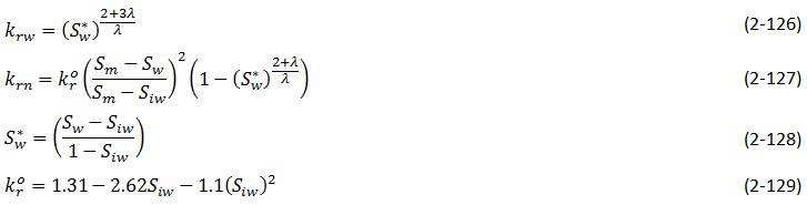
Where,
- krw = wetting phase relative permeability
- krn = non-wetting phase relative permeability
- kro = non-wetting phase rel. perm. at irreducible wetting phase saturation
- Sw* = normalized wetting phase saturation
- λ = pore size distribution index
- Sm = 1 – Sor (1 – residual non-wetting phase saturation)
- Sw = water saturation
- Siw = initial water saturation
The major difference between the Burdine solutions and the equations shown here is in the non-wetting phase equation, eq. (2‑127). The kro term is added to account for the fact that the non-wetting phase solution must be at irreducible wetting phase saturation. The other modification is the Sm term proposed by Corey in order to represent the point where the non-wetting phase first begins to flow. This is known as the critical saturation point. What this means, is that for a period at the beginning of the non-wetting phase curve, there exists a period where there is no connectivity. At the critical saturation, a minimum number of pores are connected, at which point flow is possible and the first relative permeability value can be determined. The Sm term describes the saturation at which flow is first possible and is necessary in order to calculate realistic relative permeability values.
Determining Pore Size Distribution Index
The λ value (pore size distribution index) seen in equations (2‑126) and (2‑127) is critical in calculating relative permeability. The actual number represents how uniform the pore size is in the sample/reservoir. A low value of λ (i.e. 2) indicates a wide range of pore sizes, while a high value represents a rock with a more uniform pore size distribution. Using a λ value of 2 in equations (2‑126) and (2‑127) results in the well-known Corey equations. This value is considered a general value, and is thought to represent a wide range of pore sizes. Since a λ value of 2 is so general, it is often used when nothing else is known about the reservoir. Using a λ value of 2.4 or infinity results in Wyllie’s equation for 3 rock categories[fusion_builder_container hundred_percent=”yes” overflow=”visible”][fusion_builder_row][fusion_builder_column type=”1_1″ background_position=”left top” background_color=”” border_size=”” border_color=”” border_style=”solid” spacing=”yes” background_image=”” background_repeat=”no-repeat” padding=”” margin_top=”0px” margin_bottom=”0px” class=”” id=”” animation_type=”” animation_speed=”0.3″ animation_direction=”left” hide_on_mobile=”no” center_content=”no” min_height=”none”][1]:
- λ = 2 (cemented sandstones, oolotic and small-vug limestones)
- λ = 4 (poorly sorted unconsolidated sandstones)
- λ = infinity (well sorted unconsolidated sandstones)
Wyllie’s equations are used when there is some general knowledge of the geology of the reservoir.
The Corey and Wyllie equations are sufficient for approximation purposes, but in order to obtain a more accurate value of the pore size distribution index, λ can be determined empirically from capillary pressure data. The equation shown here was developed by Brooks and Corey (1964 & 1966), and relates capillary pressure to normalized wetting phase saturation:

Where,
- Pc = capillary pressure
- Pe = minimum threshold pressure
- Sw* = normalized water saturation, eq. (2‑128)
If capillary pressure data is available, eq. (2‑130) can be used to determine the pore size distribution index. A log-log plot of the capillary pressure vs the normalized water saturation should result in a straight line with a slope of –1/ λ and an intercept of Pe. This method of determining λ from experimental data is preferable to using the Wyllie or Corey relations, since the value obtained with eq. (2‑130) can actually be backed up with hard data.
Example 2‑9[2]
For a water wet reservoir with Swi = 0.16 and residual gas saturation equal to 0.05, use the following capillary pressure data to find the relative permeability data.
| Pc ( Sw ) | Sw | Pc ( Sw ) | Sw |
| 0.5 | 0.965 | 8 | 0.266 |
| 1 | 0.713 | 16 | 0.219 |
| 2 | 0.483 | 32 | 0.191 |
| 4 | 0.347 | 300 | 0.16 |
Solution
Step 1: Calculate Normalized Water Saturation (Sw*), using eq. (2-130)
| Pc ( Sw ) | Sw | Sw* | Pc ( Sw ) | Sw | Sw* |
| 0.5 | 0.965 | 0.958 | 8 | 0.266 | 0.126 |
| 1 | 0.713 | 0.658 | 16 | 0.219 | 0.070 |
| 2 | 0.483 | 0.385 | 32 | 0.191 | 0.037 |
| 4 | 0.347 | 0.223 | 300 | 0.16 | 0.000 |
Step 2: Deterimne λ by Plotting LogPc vs. LogSw*
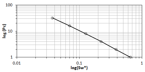
Recall eq.(2‑130), Slope of the graph is –1/ λ = -1.25, Therefore, λ = 0.8
Step 4: Calculating Non-Wetting Phase Relative Permeability at Irreducible Wetting Phase Saturation ( kro ),
Recall eq. (2‑129), kro = 0.919 and Sm = 0.95 = 1-Srg.
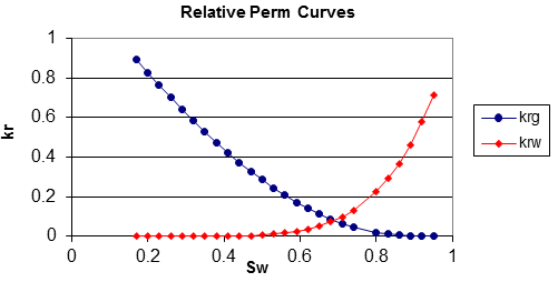
Step 5: Calculating Relative Perm Values, Recall equations (2‑126) and (2‑127) to find the relative permeability of the respective phases at various water saturations:
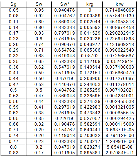
Then plot krg and krw vs. Sw in order to display the information in its most typical form:
Hornarpour Correlations
A different technique was approached by Hornarpour et al. in order to come up with correlations to estimate relative permeability. Instead of attempting to solve the problem theoretically, Hornarpour developed an entirely empirical solution to the problem. Data from numerous different fields around the world was gathered, and stepwise linear regression analysis was used to come up with mathematical descriptions to match the actual data. Data sets came from Canada, U.S., Alaska and the Middle East. The data sets were classified as either carbonate or non-carbonate and also broken up into wettability and property ranges. In this manner, equations were developed for numerous different reservoir conditions.
In order to use the Hornarpour correlation, a general understanding of the reservoir is required. Namely the fluids in the system, a rough description of the geology, the wettability and the range of rock properties and fluid saturations in the reservoir. This information is then used to determine which set of equations are to be utilized in calculating the wetting and non-wetting phase relative permeability. Hornarpour’s paper[3] provides all the necessary details (tables and equations) that are required for this method.
Comparison of Empirical Methods
Out of the methods discussed here, the most accurate results are obtained from the method in which the pore size distribution index is determined experimentally, and is then utilized in equations (2‑126) and (2‑127) for drainage relative permeability. The other methods (Corey, Wylie and Hornarpor) rely a great deal on general estimates of the reservoir conditions. For example, in the Hornarpor correlations the only choices available for geology are either carbonate or non-carbonate. Since the description of the reservoir in these methods is so vague, it is uncertain how accurate the results obtained from them can be with respect to the actual reservoir conditions. Conversely, the pore size distribution index is determined experimentally and there is hard data to back up the results.
Other Methods
Since relative permeability is such an important topic, numerous individuals have devoted their lives to determining methods to estimate relative permeability values. As such, there are numerous different techniques and methods that are used to calculate relative permeability. For example, relative permeability can be calculated through field data and analysis of pressure data. Some of the other methods not discussed in detail include theoretical models such as Naar-Wygal’s and Naar-Henderson (1961), which are for imbibition processes. The Burdine equations discussed here are for drainage calculations only.
Overall Comparison of Methods
As discussed, there are many different ways, in which relative permeability values can be estimated, from rigorous laboratory measurements, to “quick and dirty” calculations. With all of these methods available, the question as to which method should be used becomes extremely important. Like most things in the reservoir-engineering world, all of the options have their advantages and disadvantages. The only way to make a sound decision is to see what is best for the given situation, and weigh the options accordingly. For example, if relative permeability data is required for a major discovery in the North Sea, then chances are good that you would decide to spend the money to get an excellent core sample in order to run a rigorous steady-state test on it. Conversely, if data for a mature oil field is required then a quick calculation or displacement test would be sufficient for your purposes. As always, economics and practicality will be the overriding factor in deciding what sort of method to use in order to estimate relative permeability values.
[fusion_separator top=”25″/]
[fusion_builder_row_inner][fusion_builder_column_inner type=”1_2″ last=”no”]
[/fusion_builder_column_inner]
[fusion_builder_column_inner type=”1_2″ last=”yes”]
CAPILLARY PRESSURE AND WETTABILITY >>
[/fusion_builder_column_inner][/fusion_builder_row_inner]
[fusion_separator top=”35″/]
References
[2] International Petroleum Consultants, “Fundamentals of Relative Permeability”, Mobil Oil Indonesia Course Notes, 1985.
Questions?
If you have any questions at all, please feel free to ask PERM! We are here to help the community.[/fusion_builder_column][/fusion_builder_row][/fusion_builder_container]