Fundamentals of Fluid Flow in Porous Media

 

Chapter 5

Miscible Displacement

The Convection-Dispersion Model with Adsorption

The convection-dispersion equation has frequently been used with a sink or source term to account for solute adsorption and desorption at the solid/liquid interface. Adsorption during flow through porous media is of interest in a number of disciplines, such as adsorptive separation processes, chromatography, soil science, and improved oil recovery. A large body of literature on the subject exists.

The term “adsorption” refers to physical (not chemical) bonding. If a solute has a higher affinity for the solid in a porous medium than for the bulk fluid, the concentration of solute near the solid surface will be higher than in the bulk fluid. Adsorption is an equilibrium process. Solute molecules are constantly exchanged between bulk and adsorbed phases, but, at equilibrium, the average concentration of solute in the bulk and adsorbed phases is constant. The most thermodynamically consistent approach to describing adsorption is the Gibbs surface excess (Schay, 1969; Sircar and Myers, 1970, 1971; Sircar et al., 1972; Larionov and Myers, 1971; Everett, 1973; Chattoraj and Birdi, 1984; Sircar, 1985). The surface excess is defined as the excess of solute near an interface over the amount that would be present if the interface had no preference for the solute. The surface excess concept can be applied to liquids and gases, and to different kinds of interfaces (solid/liquid, solid/gas, liquid/liquid, liquid/gas). The surface excess concept has been incorporated into the convection-dispersion model by Huang and Novosad (1986) and Mannhardt and Novosad (1988, 1990).

Adsorption depends on fluid phase composition (or gas pressure) and on temperature. The dependence of adsorption on concentration (or pressure), at constant temperature, is given by an adsorption isotherm. A large number of adsorption isotherms for gases and liquids on solid surfaces is available in the literature. A discussion of some of these can be found in Adamson’s (1990) text on the physical chemistry of surfaces. The choice of adsorption isotherm and adsorption kinetics is obviously system-specific and should reflect the interfacial chemistry and physics of the system of interest. However, the choice has often been empirical and based on considerations of simplicity or fitting of experimental data. Only one simple example of a commonly used adsorption model, the Langmuir model, will be discussed here. A large number of adsorption models that have appeared in the petroleum literature are summarized in a review by Mannhardt and Nasr-El-Din (1994).

A second order reversible rate expression that has been widely used is given by Langmuir rate-controlled adsorption, also sometimes referred to as “bilinear adsorption kinetics:”

where q is amount adsorbed, q_max is the maximum adsorptive capacity of the adsorbent, and k₁ and k₂ are rate constants of adsorption and desorption, respectively.

At equilibrium, ϑq / ϑt = 0, and Equation 5‑95) becomes:

Where,

a = q_max(K₁ / K₂ ),

b = ( K₁ / K₂ )

and a and b are the Langmuir constants. Equation (5‑96) is the Langmuir adsorption isotherm. Its typical shape is shown in Figure 5‑64. At low concentration, q≈ac, and the isotherm becomes nearly linear. At high concentration, the isotherm asymptotically approaches q_max.

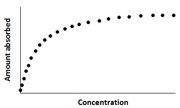
Figure 5-64: Typical Shape of a Langmuir Adsorption Isotherm

The Langmuir equilibrium isotherm has been widely used for adsorption at gas/solid and liquid/solid interfaces because it describes the general shape of many adsorption isotherms adequately. While it contains too many simplifying assumptions to represent many real adsorption systems, it has retained great utility because of its simplicity. Many adsorption processes from gases and liquids can be modeled by the Langmuir equation despite the fact that the simplifying assumptions made in its derivation are rarely met.

With adsorption, the one-dimensional convection-dispersion equation becomes:

Where,

q = amount adsorbed (mass of solute per unit mass of solid),

φ = porosity,

ρ_r = solid (grain) density (mass of solid per unit volume).

In addition to initial and boundary conditions, a condition specifying the initial value of adsorption is required; often q = 0 at t = 0. An adsorption model, such as the Langmuir model, is also required to describe q in eq. (5‑97). When adsorption kinetics are important, adsorption is modelled as a dynamic process by substituting eq. 5‑95) (or alternative models) for  in eq. (5‑97). When adsorption is fast compared to convective mass transfer, adsorption equilibrium can be assumed. Then,

Substituting Equation (5‑98) into Equation (5‑97) gives:

where dq / dc is the slope of the adsorption isotherm. The factor multiplying the time derivative is frequently referred to as “retardation factor,” since it is a measure of the rate of propagation of an adsorbing versus a non-adsorbing solute. Any adsorption isotherm can be substituted for dq / dc. Using again the Langmuir adsorption isotherm (eq. (5‑96)) as an example, eq. (5‑99) becomes:

Adsorption models with Langmuir rate-controlled or equilibrium adsorption constitute non-linear partial differential equations. No analytical solutions are available, and numerical solutions have to be resorted to. However, at low concentration, the Langmuir adsorption isotherm becomes nearly linear. When q = ac, the adsorption model can be solved analytically with boundary conditions for infinite, semi-infinite and finite domains (Gershon and Nir, 1969; Satter et al.; 1980, van Genuchten and Alves, 1982).

Transport of surfactants in petroleum reservoir rocks or of pollutants in ground water has frequently been modelled using Langmuir adsorption, for example by Gupta and Greenkorn (1973), Trogus et al. (1977), Shuler (1978), Satter et al. (1980), Ramirez et al. (1980), Ziegler and Handy (1981), Foulser et al. (1989), Novosad et al. (1986), and Huang and Novosad (1986). The shape of a concentration profile for an adsorbing system is determined by the relative magnitudes of the rates of dispersion, convection, adsorption, and desorption, and by the adsorptive capacity of the rock. The effect of these groups on effluent profiles has been discussed in detail by Satter et al. (1980) using Langmuir adsorption. Examples of concentration profiles for a slug of an adsorbing solute injected into a porous medium that is fully saturated with solvent, obtained using the model of Mannhardt and Novosad (1988), are shown in Figure 5‑65.

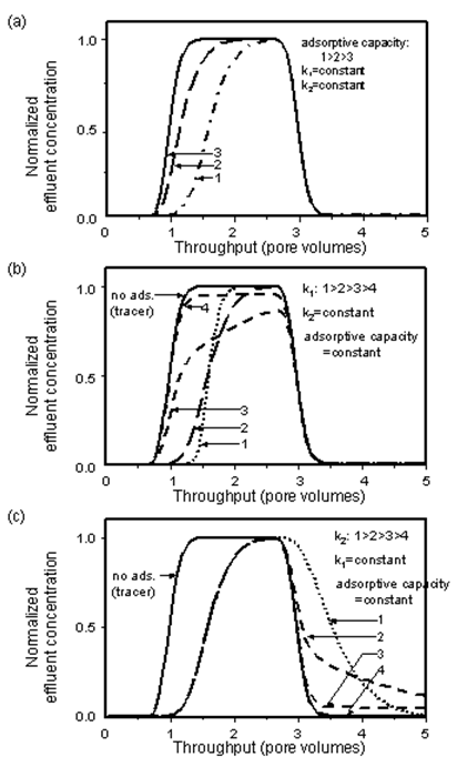
Figure 5-65: Effect of Adsorption Model Parameters on Adsorbate Effluent Conditions: (a) Effect of Adsorptive Capacity, (b) Effect of Rate of Adsorption, (c) Effect of rate of Desorption

Increasing the adsorptive capacity of the solid delays breakthrough of the adsorbing solute at the porous medium outlet. When the rate of adsorption is high compared to convective mass transfer, equilibrium is reached at the solid surface. The leading edge of the concentration profile is similar in shape to the zero adsorption (tracer) case, but is displaced towards higher injection volumes, as some of the solute is held back on the solid surfaces. When the rate of adsorption is decreased, solute breakthrough occurs earlier and the profile becomes skewed. At very low rates of adsorption, solute breakthrough almost coincides with tracer breakthrough, and the profile again becomes steep, but the solute concentration becomes nearly constant at a value lower than the injected concentration.

The kinetics of desorption mirror the kinetics of adsorption, at the trailing edge of the solute slug. The concentrations now reflect injection of solvent into a porous medium that is fully saturated with solute. When desorption is very slow, tracer and solute are produced almost simultaneously. As the rate of desorption increases, solute is eluted for longer periods of time than tracer, as the adsorbed solute is released from the solid surfaces. At high rates of desorption, solute is eluted quickly until, at very high desorption rates, all the adsorbed solute is recovered in the effluent over a short injection volume.

The validity of the adsorption model with Langmuir rate-controlled or equilibrium adsorption (or any other adsorption term) can be tested by comparing predicted to experimental effluent concentrations of adsorbing chemicals from porous media, as has frequently been done with surfactant solutions used in improved oil recovery. The model parameters, which include the dispersion coefficient, Langmuir constants (a and b), and rate constants of adsorption and desorption, can be determined by fitting experimental effluent data. Alternatively, some of the parameters may be measured independently. For example, the dispersion coefficient may be found from tracer data (Foulser et al., 1989), or by measuring surfactant dispersion in a porous medium whose surfaces have been pre-saturated with surfactant (Friedman, 1976; Shuler, 1978). The Langmuir constants may be obtained from adsorption isotherms measured statically in test tubes, or by performing material balance calculations in dynamic test runs at different input concentrations (Trogus et al., 1977; Ramirez et al., 1980; Ziegler and Handy, 1981). This would leave only the rate constants as adjustable parameters for fitting of adsorbate effluent profiles.

An adsorption isotherm such as eq. (5‑96) describes the dependence of adsorption on concentration at equilibrium. The dependence of adsorption on time at a fixed concentration can be obtained by solving the appropriate rate equation. With initial condition q=q₀, solving eq. 5‑95) gives the time dependence of adsorption assuming Langmuir kinetics, as follows:

Whether adsorption equilibrium can be assumed (eqs (5‑99) or (5‑100)) or the kinetics of adsorption need to be taken into account (eq. (5‑97)) depends on the relative rates of adsorption and convective mass transport.

Some Other Forms of the Convection-Dispersion Model

These notes have discussed some examples of models used to describe various mass transfer processes during miscible displacement in porous media. Other mechanisms, or combinations of mechanisms, can be encountered and described by similar models. Some of these mechanisms include

• chemical reaction,
• precipitation,
• ion exchange,
• inaccessible pore volume (capacitance with no mass transfer into stagnant pore space), and
• partitioning of species between immiscible phases.

 

Laboratory core floods are commonly used to provide information about these mechanisms. The effluent profiles from core floods can provide a “finger print” of the porous medium and its interaction with the fluids flowing through it. Thus, a core flood can be designed to yield information on

• the porous medium (dispersion, heterogeneity, capacitance, ion exchange, adsorption, inaccessible pore volume),
• the fluids, solutes, or chemical species flowing through the porous medium (dispersion, adsorption, reaction, partitioning, precipitation, ion exchange), and
• the distribution of immiscible phases in the porous medium (wetting, connectivity, phase saturation, trapping).