
Fundamentals of Fluid Flow in Porous Media
Chapter 4
Immiscible Displacement
Water Injection Oil Recovery Calculations: Mobility Ratio Effect
The basic mechanics of oil displacement by water can be understood by considering the mobilities of the separate fluids[fusion_builder_container hundred_percent=”yes” overflow=”visible”][fusion_builder_row][fusion_builder_column type=”1_1″ background_position=”left top” background_color=”” border_size=”” border_color=”” border_style=”solid” spacing=”yes” background_image=”” background_repeat=”no-repeat” padding=”” margin_top=”0px” margin_bottom=”0px” class=”” id=”” animation_type=”” animation_speed=”0.3″ animation_direction=”left” hide_on_mobile=”no” center_content=”no” min_height=”none”][1]. The mobility of any fluid is defined as:

Where, k is absolute permeability and kr is relative permeability.
The manner in which water displaces oil is illustrated in Figure 4‑14 for both an ideal and non-ideal linear horizontal waterflood.
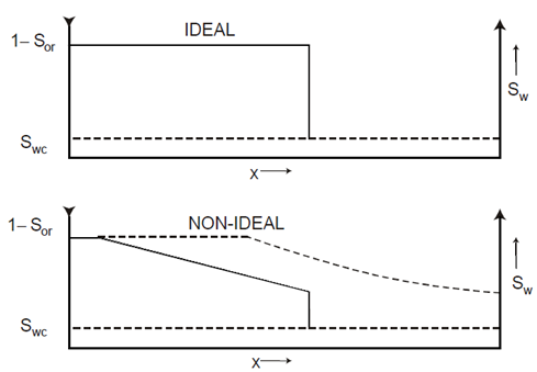
Figure 4-14: Water Saturation Distribution as a Function of Distance between Injection and Production Wells for (a) Ideal or Piston-like Displacement and (b) Non-ideal Displacement
In the ideal case there is a sharp interface between the oil and water. Ahead of this, oil is flowing in the presence of connate water 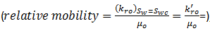 , while behind the interface water alone is flowing in the presence of residual oil
 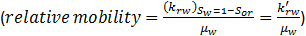 . This favorable type of displacement will only occur if the ratio

Where, M is known as the end point mobility ratio and, since both k‘ro and k‘rw are the end point relative permeabilities, is a constant.
If M ≤ 1 it means that, under an imposed pressure differential, the oil is capable of travelling with a velocity equal to, or greater than, that of the water. Since it is the water which is pushing the oil, there is therefore, no tendency for the oil to be by-passed which results in the sharp interface between the fluids.
The displacement shown in Figure 4‑14(a) is, for obvious reasons, called “piston-like displacement“. Its most attractive feature is that the total amount of oil that can be recovered from a linear reservoir block will be obtained by the injection of the same volume of water. This is called the movable oil volume where:

The non-ideal displacement depicted in Figure 4‑14(b), which unfortunately is more common in nature, occurs when M > 1. In this case, the water is capable of travelling faster than the oil and, as the water pushes the oil through the reservoir, the latter will be by-passed. Water tongues or fingers develop leading to the unfavorable water saturation profile.
Ahead of the water front oil is again flowing in the presence of connate water. This is followed, in many cases, by a waterflood front, or shock front, in which there is a discontinuity in the water saturation. There is then a gradual transition between the shock front saturation and the maximum saturation Sw = 1 − Sor. The dashed line in Figure 4‑14(b) depicts the saturation distribution at the breakthrough time. In contrast to the piston-like displacement, not all of the movable oil will have been recovered at this time. As more water is injected, the plane of maximum water saturation ( Sw = 1 − Sor ) will move slowly through the reservoir until it reaches the producing well at which time the movable oil volume has been recovered. Unfortunately, in typical cases it may take five or six MOV’s of injected water to displace the one MOV of oil. At a constant rate of water injection, the fact that much more water must be injected, in the unfavorable case, protracts the time scale attached to the oil recovery and this is economically unfavourable. In addition, pockets of by-passed oil are created which may never be recovered.
An even more significant parameter for characterizing the stability of Buckley Leverett displacement is the shock front mobility ratio, Ms, defined as:
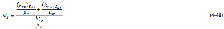
in which the relative permeabilities in the numerator are evaluated for the shock front water saturation, Swƒ. Hagoort[2] has shown, using a theoretical argument backed by experiment, that Buckley-Leverett displacement can be regarded as stable for the less restrictive condition that Ms < 1. If this condition is not satisfied there will be severe viscous channeling of water through the oil and breakthrough will occur even earlier than predicted using the Welge technique.
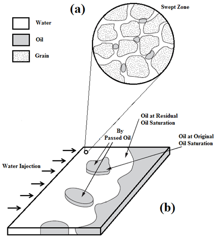
Figure 4-15: (a) Microscopic Displacement (b) Residual Oil Remaining After a Water Flood
Example 4-2[3]
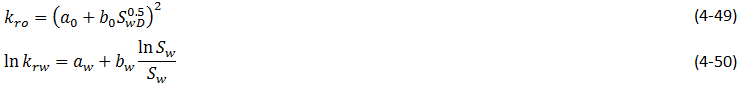
A thin reservoir zone (8 ft thick) is to be opened in several wells to production. The oil from this zone is expected to have a viscosity of 2.36 cp at reservoir temperature. Because the oil is essentially dead, it will be necessary to supplement the reservoir energy to produce oil at economical rates. A waterflood is under consideration. Relative permeability data from an adjacent interval have been correlated with water saturation by use of eqs (4‑49) and (4‑50). Log calculations indicate that the initial water saturation should be 0.136. A residual oil saturation of 0.325 was obtained on cores from a geologically similar interval.
Where,
- Calculate the waterflood recovery (PV) when the saturation at end face is equal to 0.54. The viscosity of water at reservoir temperature is 0.63 cp.
- Calculate the oil recovery when water oil ratio (WOR) =27.57.
- Calculate post breakthrough performance
Solution
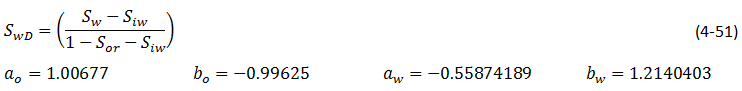
The first step is drawing ƒw – Sw curve according to eq. (4‑7). Eqs (4‑49) and (4‑50) are used to find relative permeabilities data that are needed for ƒw calculations:
| Sw | SwD | kro | krw | ƒw | Sw | SwD | kro | krw | ƒw |
| 0.1500 | 0.0260 | 0.7058 | 0.0000 | 0.0000 | 0.4500 | 0.5826 | 0.0577 | 0.0663 | 0.8115 |
| 0.2000 | 0.1187 | 0.4322 | 0.0000 | 0.0003 | 0.5000 | 0.6753 | 0.0331 | 0.1063 | 0.9232 |
| 0.2500 | 0.2115 | 0.2943 | 0.0007 | 0.0086 | 0.5500 | 0.7681 | 0.0163 | 0.1528 | 0.9724 |
| 0.3000 | 0.3043 | 0.2035 | 0.0044 | 0.0746 | 0.6000 | 0.8609 | 0.0058 | 0.2034 | 0.9924 |
| 0.3500 | 0.3970 | 0.1391 | 0.0150 | 0.2876 | 0.6500 | 0.9536 | 0.0008 | 0.2558 | 0.9992 |
| 0.4000 | 0.4898 | 0.0921 | 0.0354 | 0.5905 | 0.6750 | 1.0000 | 0.0000 | 0.2821 | 1.0000 |
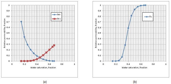
Figure 4-16: (a) Relative Permeability Curves, (b) Fractional Flow Curve
[fusion_builder_row_inner][fusion_builder_column_inner type=”1_2″ last=”no”]
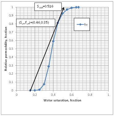
Figure 4-17: Graphical Determination of Front Saturation and Water Fractional Flow
[/fusion_builder_column_inner]
[fusion_builder_column_inner type=”1_2″ last=”yes”]
To find the water saturation at the front and average water saturation at breakthrough time, a tangent is drawn from initial water saturation point ( Swi , 0 ) = ( 0.15 , 0 ) to the ( ƒw vs. Sw ) curve. Line touches the curve at the front saturation point. According to Figure 4‑17, the front point coordination is: ( Swƒ , ƒwƒ ) = ( 0.46 , 0.85 ).
Average saturation at breakthrough time could be found by continuing the tangent line to the line ƒw = 1. According to the Figure 4‑17 average water saturation at breakthrough time is: Swbt = 0.516.
[/fusion_builder_column_inner][/fusion_builder_row_inner]
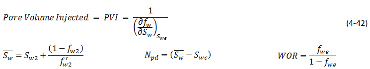
The pore volume injected of water (PVI) up to breakthrough time that is equal to the produced oil until this time (fluids are assumed to be incompressible), could be calculated using either eq. (4‑40) or (4‑44):
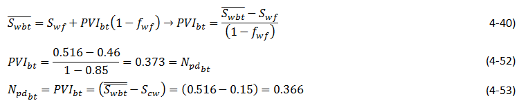
The difference between two results (from eqs (4‑52) and (4‑53)) is resulted from the graphical reading of the front saturation and fractional flow. So the water flood recovery at breakthrough time is around 37%.
To calculate oil recovery after breakthrough time when producing WOR is, using the following equation to convert WOR to fw:

According to Wedge equation, we should pass a tangent through the ( ƒw – Sw ) curve at point Sw = 0.54 , ƒw = 0.965 , see Figure 4‑18.
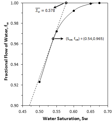
Figure 4-18: Fractional Flow of Water vs. Water Saturation
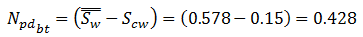
The tangent line cut the ƒw = 1 line at Sw = 0.578, which is the average saturation in the medium when Sw at the producing (end) face is 0.54. Npd could be found using eq. (4‑53):
The following calculations are done to find post breakthrough performance:
Using the fractional flow curve and these equations, the following table is generated for saturation higher than the front saturation ( Swƒ = 0.46 ):
| Swe | ƒwe | dƒw / dSw | PVI | Sw | Npd | WOR |
| 0.47 | 0.8668 | 2.1854 | 0.4576 | 0.5310 | 0.3810 | 6.5050 |
| 0.49 | 0.9073 | 1.6538 | 0.6047 | 0.5460 | 0.3960 | 9.7918 |
| 0.52 | 0.9480 | 1.0440 | 0.9578 | 0.5698 | 0.4198 | 18.2301 |
| 0.55 | 0.9724 | 0.6232 | 1.6046 | 0.5943 | 0.4443 | 35.1883 |
| 0.57 | 0.9827 | 0.4275 | 2.3390 | 0.6105 | 0.4605 | 56.8196 |
| 0.59 | 0.9898 | 0.2856 | 3.5012 | 0.6257 | 0.4757 | 97.0241 |
| 0.62 | 0.9962 | 0.1471 | 6.7995 | 0.6458 | 0.4958 | 262.0579 |
| 0.65 | 0.9992 | 0.0615 | 16.2719 | 0.6631 | 0.5131 | 1239.4319 |
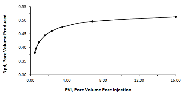
Figure 4-19: Dimensionless Pore Volume Oil Recovery vs. Dimensionless Pore Volume Water Injection
Example 4-3[1]
Oil is being displaced by water in a horizontal, direct line drive under the diffuse flow condition. The rock relative permeability functions for water and oil are listed in following table:
| Sw | krw | kro | Sw | krw | kro |
| 0.20 | 0.000 | 0.800 | 0.55 | 0.100 | 0.120 |
| 0.25 | 0.002 | 0.610 | 0.60 | 0.132 | 0.081 |
| 0.30 | 0.009 | 0.470 | 0.65 | 0.170 | 0.050 |
| 0.35 | 0.020 | 0.370 | 0.70 | 0.208 | 0.027 |
| 0.40 | 0.033 | 0.285 | 0.75 | 0.251 | 0.010 |
| 0.45 | 0.051 | 0.220 | 0.80 | 0.300 | 0.000 |
| 0.50 | 0.075 | 0.163 |
Pressure is being maintained at its initial value for which:

Compare the values of the producing watercut (at surface conditions) and the cumulative oil recovery at breakthrough for the following fluid combinations.
| Case | Oil Viscosity (cp) | Water Viscosity (cp) |
| 1 | 50 | 0.5 |
| 2 | 5 | 0.5 |
| 3 | 0.4 | 1.0 |
Assume that the relative permeability and PVT data are relevant for all three cases.
Solution
1) For horizontal flow the fractional flow in the reservoir is

While the producing watercut at the surface, ƒws , is

Where the rates are expressed in rb / d. Combining the above two equations leads to an expression for the surface watercut as:

The fractional flow in the reservoir for the three cases can be calculated as follows:
| Fractional Flow ( ƒw ) | |||||||
| Case 1 | Case 2 | Case 3 | |||||
| Sw | krw | kro | kro / krw | μw / μo = 0.01 | μw / μo = 0.1 | μw / μo = 2.5 | |
| 0.20 | 0.000 | 0.800 | ∞ | 0 | 0 | 0 | |
| 0.25 | 0.002 | 0.610 | 305.000 | 0.247 | 0.032 | 0.001 | |
| 0.30 | 0.009 | 0.470 | 52.222 | 0.657 | 0.161 | 0.008 | |
| 0.35 | 0.020 | 0.370 | 18.500 | 0.844 | 0.351 | 0.021 | |
| 0.40 | 0.033 | 0.285 | 8.636 | 0.921 | 0.537 | 0.044 | |
| 0.45 | 0.051 | 0.220 | 4.314 | 0.959 | 0.699 | 0.085 | |
| 0.50 | 0.075 | 0.163 | 2.173 | 0.979 | 0.821 | 0.155 | |
| 0.55 | 0.100 | 0.120 | 1.200 | 0.988 | 0.893 | 0.250 | |
| 0.60 | 0.132 | 0.081 | 0.614 | 0.994 | 0.942 | 0.394 | |
| 0.65 | 0.170 | 0.050 | 0.294 | 0.997 | 0.971 | 0.576 | |
| 0.70 | 0.208 | 0.027 | 0.130 | 0.999 | 0.987 | 0.755 | |
| 0.75 | 0.251 | 0.010 | 0.040 | 0.999 | 0.996 | 0.909 | |
| 0.80 | 0.300 | 0.000 | 0.000 | 1.000 | 1.000 | 1.000 | |
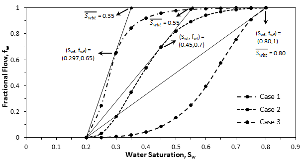
Figure 4-20: Fractional Flow Plots for Different Oil-Water Viscosity Ratios
Fractional flow plots for the three cases are shown in Figure 4‑20, and the results obtained by applying Welge’s graphical technique, at breakthrough, are listed in the following table:
| Case | Swbt | ƒwbt (Reservoir Cond.) | ƒwbt(Surface) | Swbt | Npdbt |
| 1 | 0.297 | 0.65 | 0.71 | 0.35 | 0.15 |
| 2 | 0.45 | 0.85 | 0.88 | 0.55 | 0.35 |
| 3 | 0.80 | 1.00 | 1.00 | 0.80 | 0.60 |
The results show an increment in breakthrough recovery of water injection process by increasing the water-oil viscosity ratio ( μw / μo ).
Values of M and Ms for the three cases are listed in the following. Using these data:
| Case | μo / μS | Swƒ | ( krw )Swƒ | ( kro )Swƒ | MS | M |
| 1 | 100 | 0.297 | 0.006 | 0.520 | 1.40 | 37.50 |
| 2 | 10 | 0.45 | 0.051 | 0.220 | 0.91 | 3.75 |
| 3 | 0.4 | 0.80 | 0.300 | 0.000 | 0.15 | 0.15 |
Recovery performance of water injection increases by increasing water to oil viscosity ratio, Figure 4‑21.
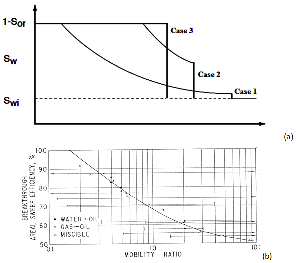
Figure 4-21: (a) Water Saturation Distribution in Systems for Different Oil/Water Viscosity Ratios (b) Areal Sweep Efficiency at Breakthrough, Five-Spot Pattern (Craig, 1980)
The typical injection/production well configurations and associated flooding patterns are shown in 4-22, including the five-spot pattern used for the results shown in 4-21.
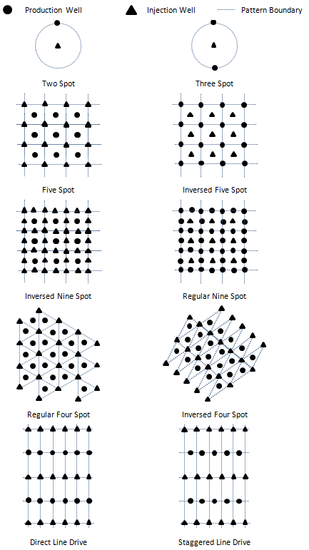
Figure 4-22: Typical Injection/Production Well Configurations and Associated Flooding Patterns
[fusion_separator top=”25″/]
[fusion_builder_row_inner][fusion_builder_column_inner type=”1_2″ last=”no”]
<< WATER INJECTION OIL RECOVERY CALCULATIONS
[/fusion_builder_column_inner]
[fusion_builder_column_inner type=”1_2″ last=”yes”]
VERTICAL AND VOLUMETRIC SWEEP EFFICIENCIES >>
[/fusion_builder_column_inner][/fusion_builder_row_inner]
[fusion_separator top=”35″/]
References
[1] “Fundamentals of Reservoir Engineering”, L.P.Dake, 1978.
[2] “Displacement Stability of Water Drives in Water Wet Connate Water Bearing Reservoirs”, Hagoort, J., 1974. Soc.Pet.Eng.J., February: 63-74. Trans. AI ME.
[3] “Enhanced Oil Recovery”, Don, W. Green, G. Paul Willhite, 1998
Questions?
If you have any questions at all, please feel free to ask PERM! We are here to help the community.[/fusion_builder_column][/fusion_builder_row][/fusion_builder_container]