Digital Core Analysis
Workflow
- Domain Preparation
- Synthetic Media Generator, or
- Imaging of Real Porous Media (micro-ct, FIB-SEM, etc)
- Modeling & Simulations
- Experiments to Calibrate
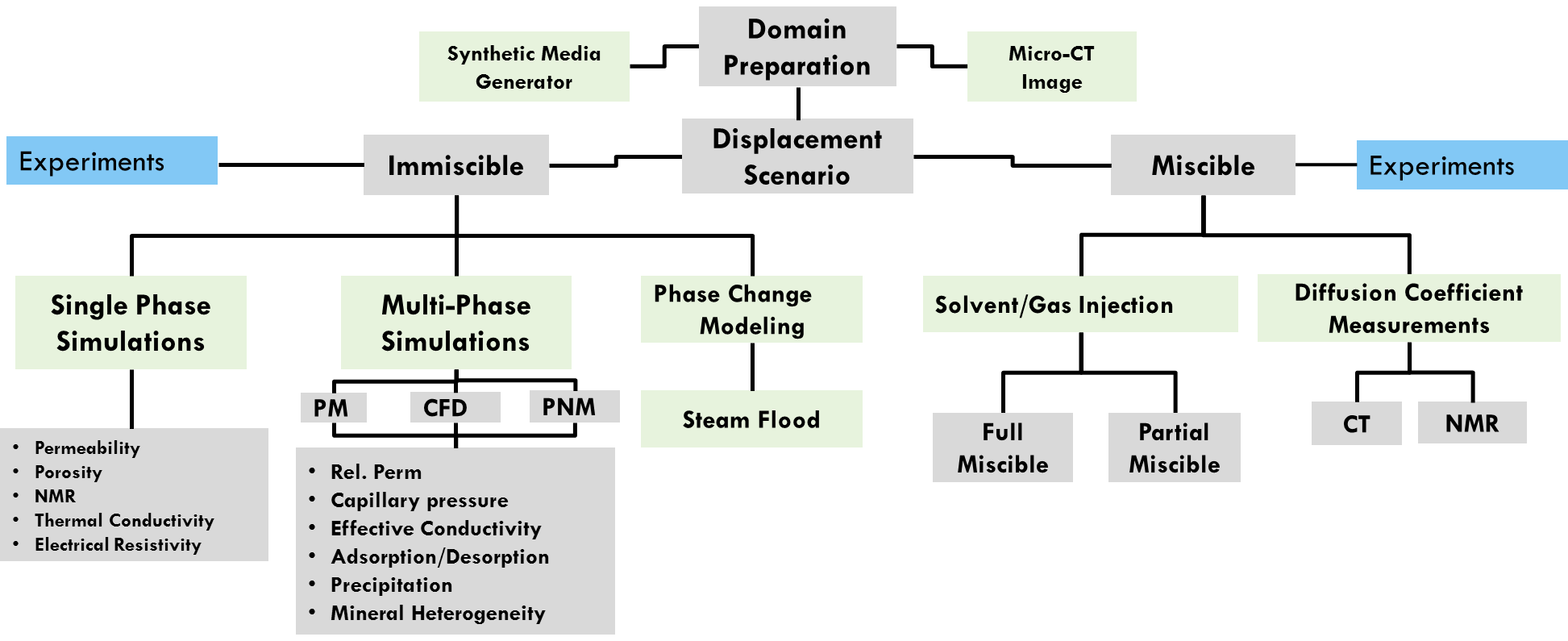
Generate Porous Media
A virtual porous media can be created from two different methods:
- Actual Imaging of the Porous Media (core) with technology such as Miro-CT or FIB-SEM (for tight core).
- Pore Size Distribution Data, which is used to create a virtual packing of particles.
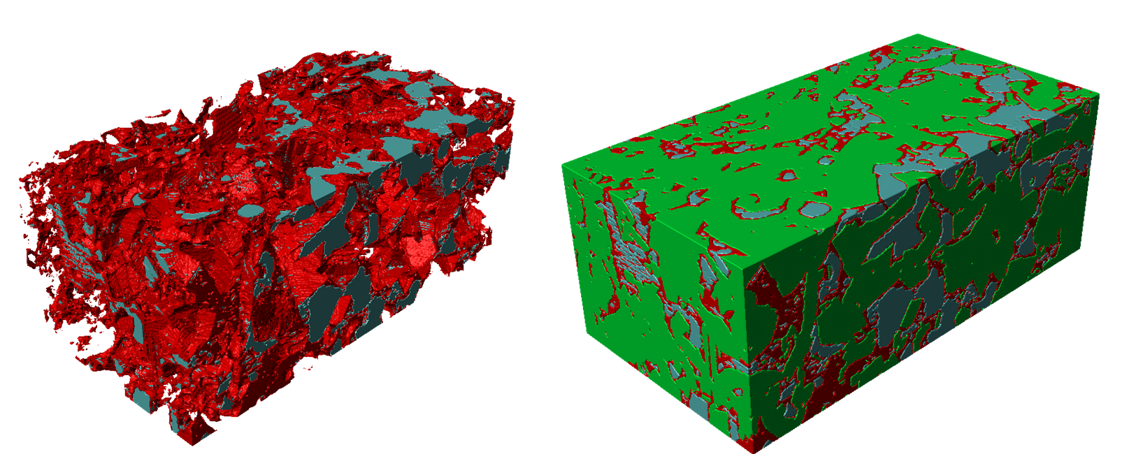
Micro-CT Images
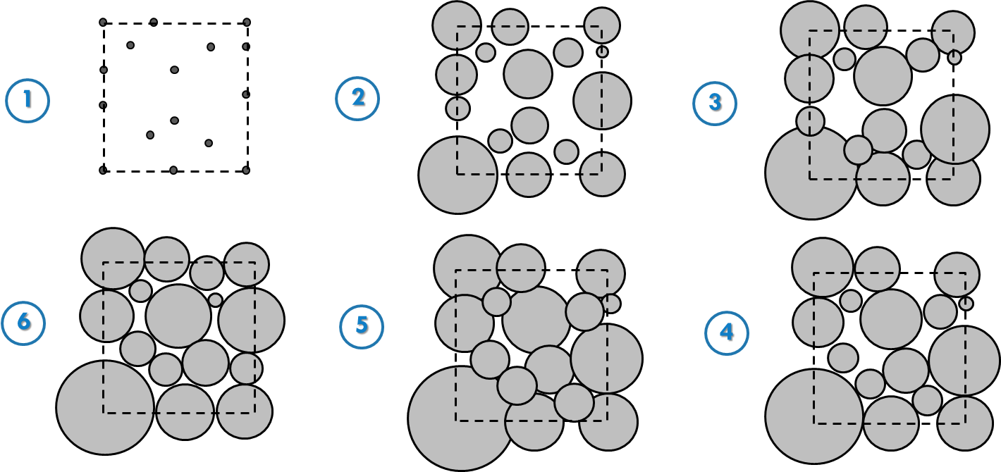
Sphere Swelling Method for Synthetically Derived Porous Media
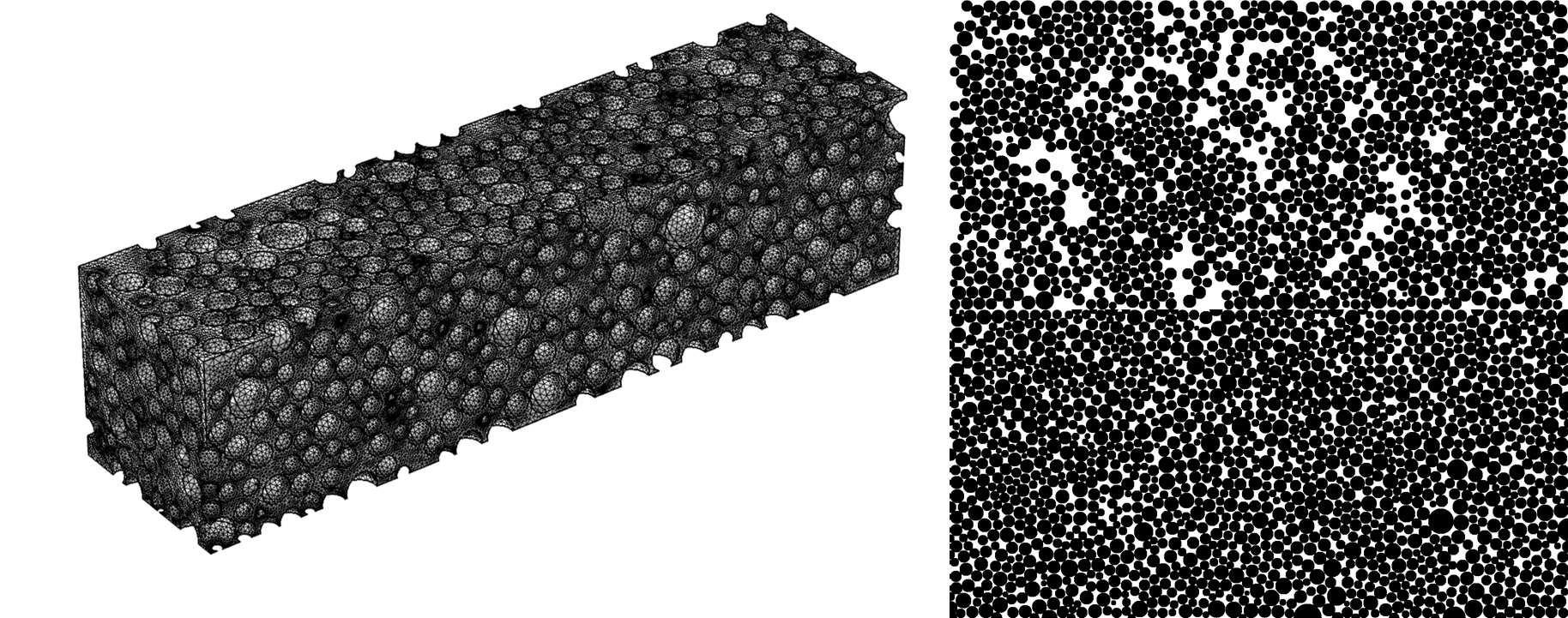
Generated Synthetic Media Examples
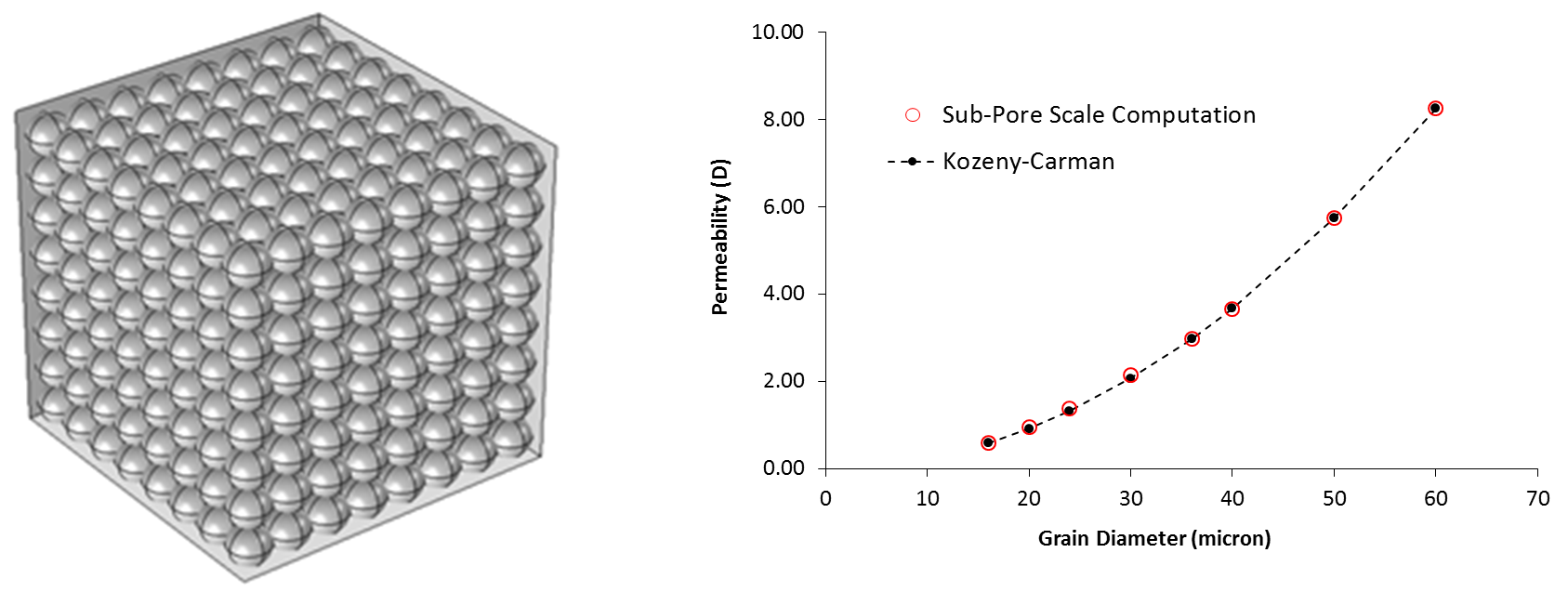
Validation of Results from Virtual Packing of Spheres
Tight Media
Simulator was modified to reduce the porosity to lower values by putting new grains to empty spaces of original generated pattern.

Multi-layered Media
- Different layer each one has its own Pore Size Distribution (PSD) and porosity
- Layering could be horizontal or vertical
- Each layer could have its own specific thickness

Single Phase Properties
First principle calculations (e.g, Navier-Stokes, Maxwell, etc) are used to derive properties such as:
- Permeability
- Porosity
- NMR spectra
- Thermal Conductivity
- Electrical Resistivity
Single Phase Flow Properties for Sandstone
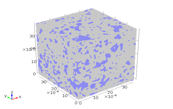
13% porosity
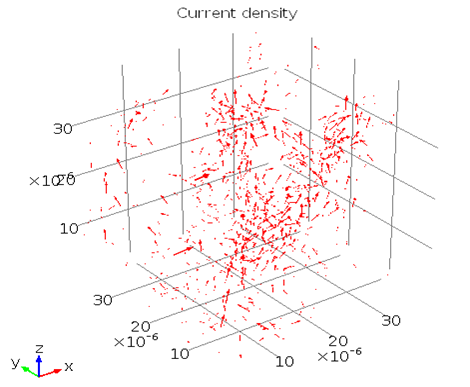
Resistivity is 80 Ω m
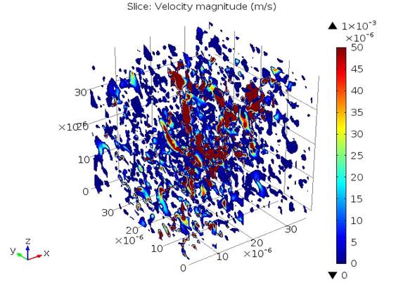
Permeability is 40 µD
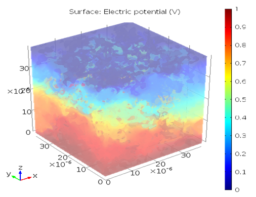
F, Archie’s Exponents
Sand pack from actual set of images. However in this case we synthetically created more grains in each 2D cross-section in order to decrease its porosity and evaluate Archie exponent shown in the below.
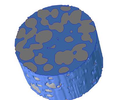
φ ≅ 50%
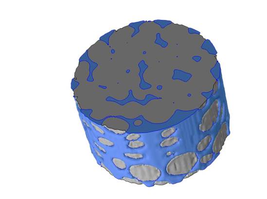
φ ≅ 18%
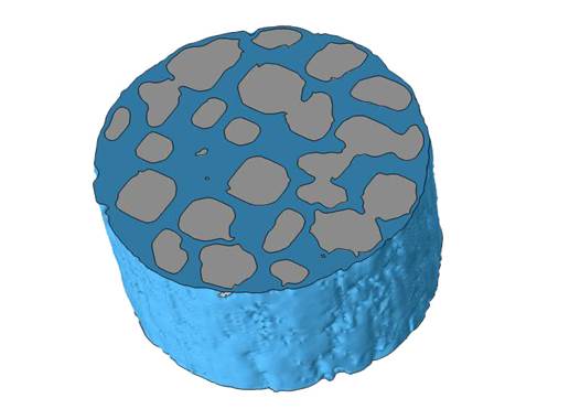
φ ≅ 42%
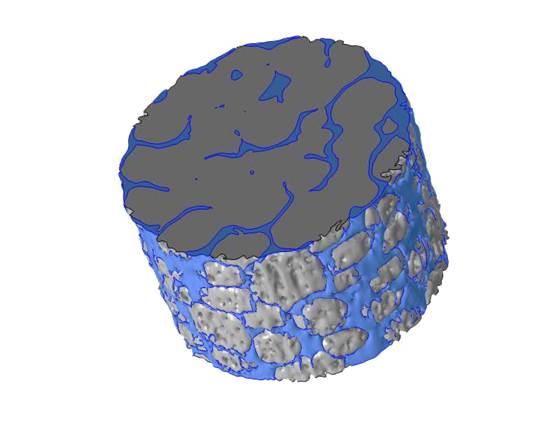
φ ≅ 8%
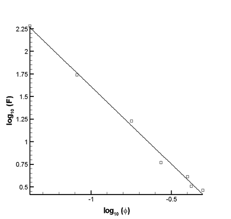
F = A “φ” ^(-m) for different φ, gives m≅1.7
Reservoir Characterization Using NMR
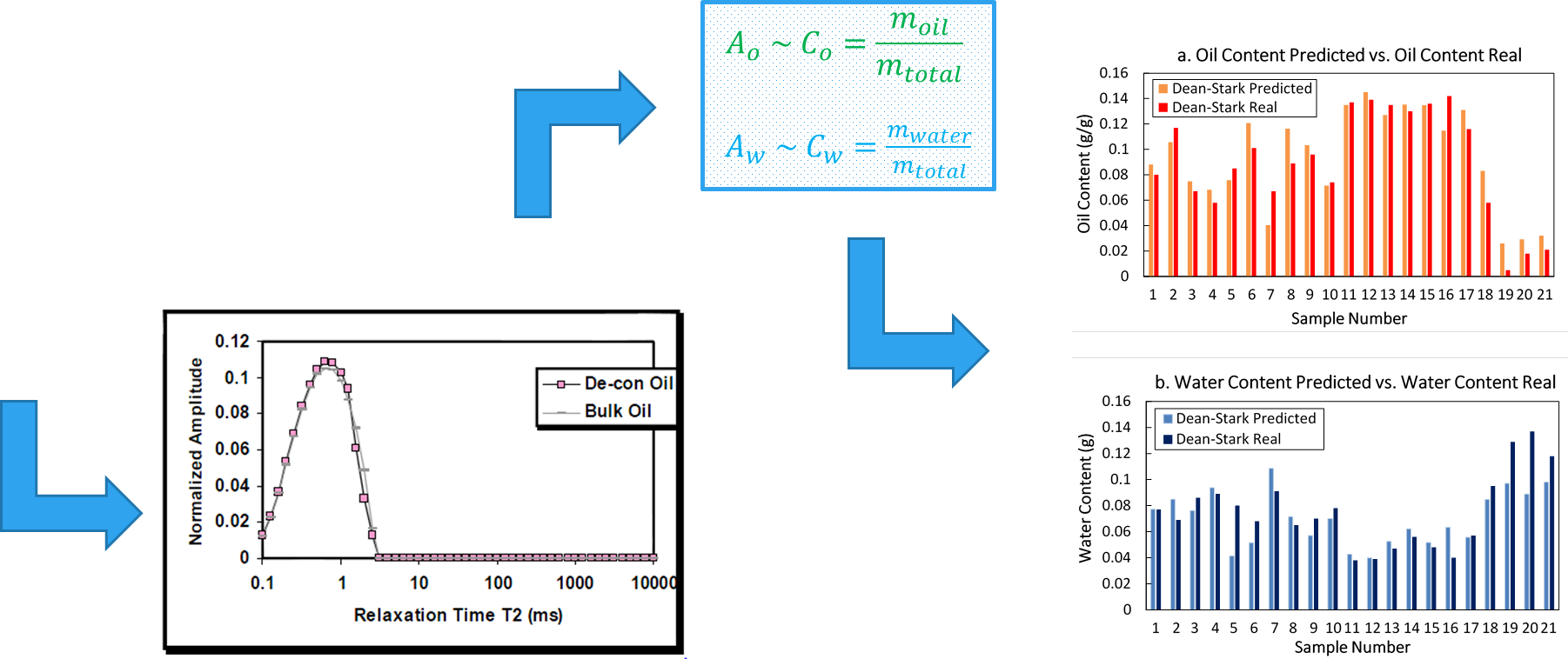
NMR Relaxation in Porous Media
- From Bloch-Torrey equations: (∂c_i)/∂t + ∇.(-D∇c_i) = – c_i/T_2B ,
- With boundary conditions: ρ_s c_i + D_i n ̂ ∇c_i = 0
- D_i: Diffusion coefficient (constant in this, however generally is tensor)
- c_i: concentration
- ρ_s: surface relaxivity and is a measure of loss of magnetization at fluid boundary S.
- T_2B is Bulk relaxation time:
For water T_2B=3.1 s, water diffusion coefficient: 2.07 x 〖10〗^(-9) m^2/s .
For Oil T_2B= 0.00122 s, Oil viscosity: 1000 cp,
Oil Diffusion coefficient: 1.3 x 〖10〗^(-12) m^2/s.
〖water-solid: ρ〗_s = 4.1 x 〖10〗^(-5) m/s, 〖oil-solid: ρ〗_s = 4.1 x 〖10〗^(-6) m/s
Water – oil interface: ρ_s= 4.1 x 〖10〗^(-7) m/s
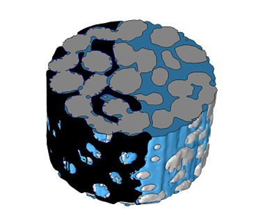
Porous media saturated if water (blue) and oil (black)
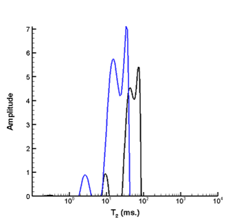
NMR spectra Fully saturated with water (blue) Fully saturated with oil (black)
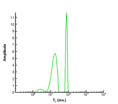
Oil-Water system resulting from addition of the different components.
Diffusion Coefficient Measurement Using Computed Tomography and Nuclear Magnetic Resonance Imaging
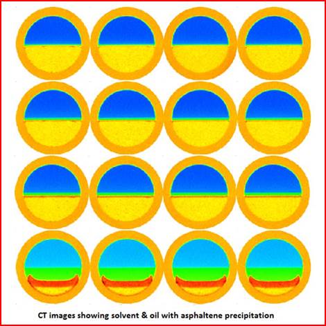
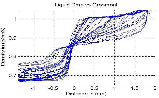
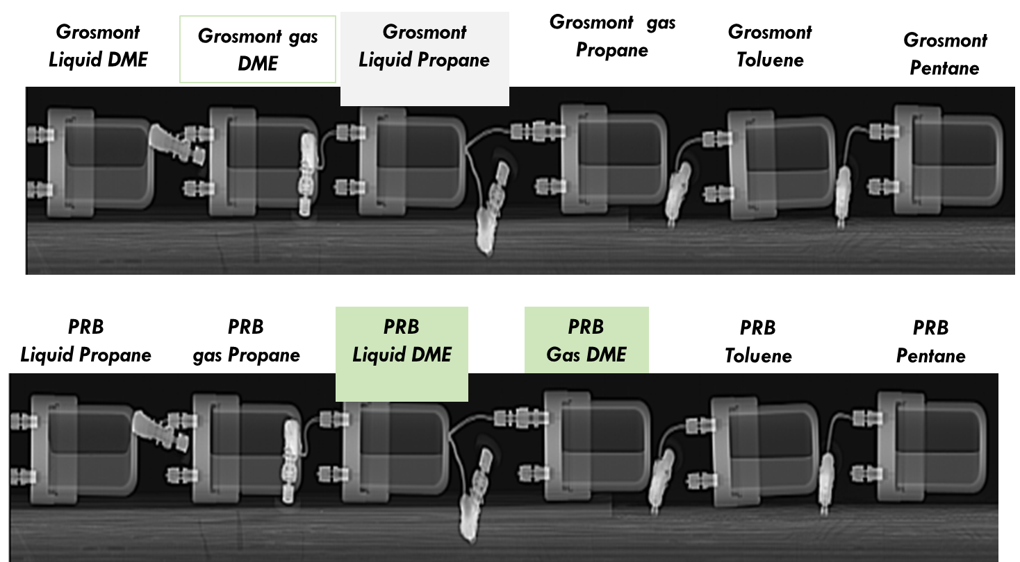
Evaluation of Diffusion of Light Hydrocarbon Solvents in Bitumen
Apparatus for MRI
- FOR LIQUID SOLVENTS CT IS MORE THAN ADEQUATE
- FOR GASEOUS SOLVENT MRI IS MORE APPROPRIATE
- BUT FIRST IT NEEDS TO BE TESTED WITH LIQUIDS
- 1-D Nuclear Magnetic Resonance Imaging (MRI) is employed to obtain diffusivity data for a toluene-heavy oil system
- “Oxford Instruments” NMR apparatus operating at a resonance frequency of 2.5MHz is used

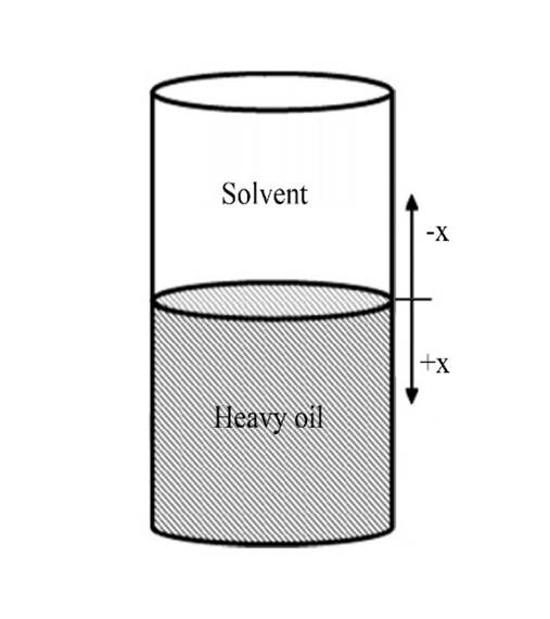
Acquiring MRI signals
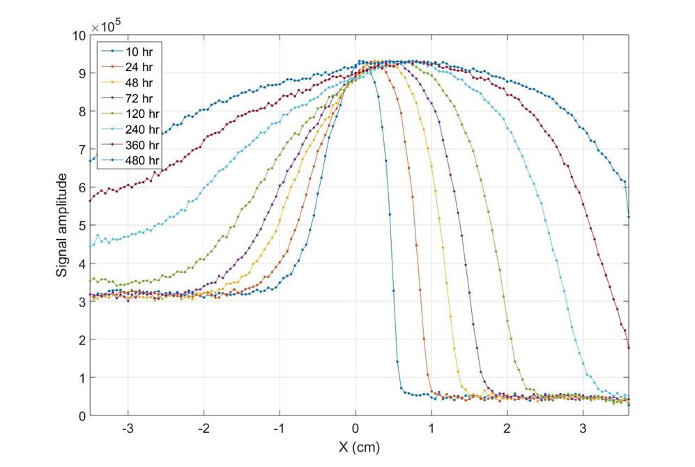
- The diffusion experiment was monitored for 20 days
- The width of the signal: the length of the sample
- The height of the signal: the amplitude in each cross section

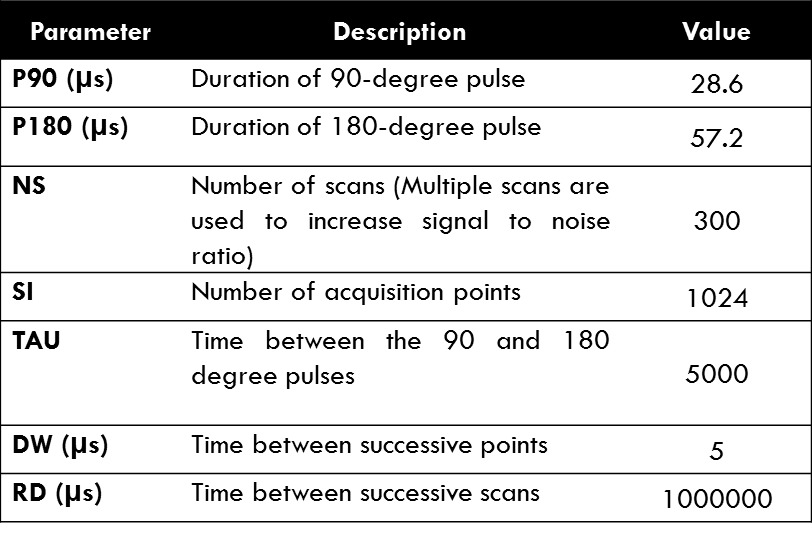
Converting MRI Signals to Concentration Profiles
MRI Signals

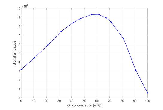
Calibration Curve

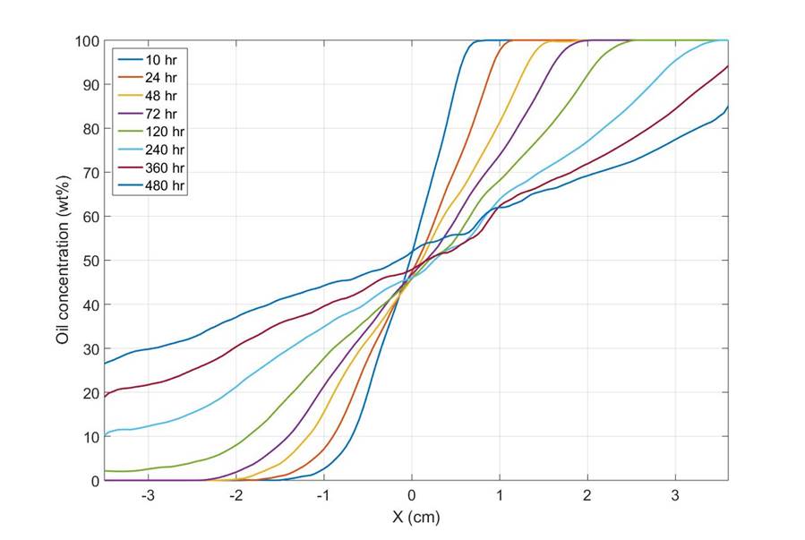
Oil concentration profiles at different mixing times
Diffusion Coefficients
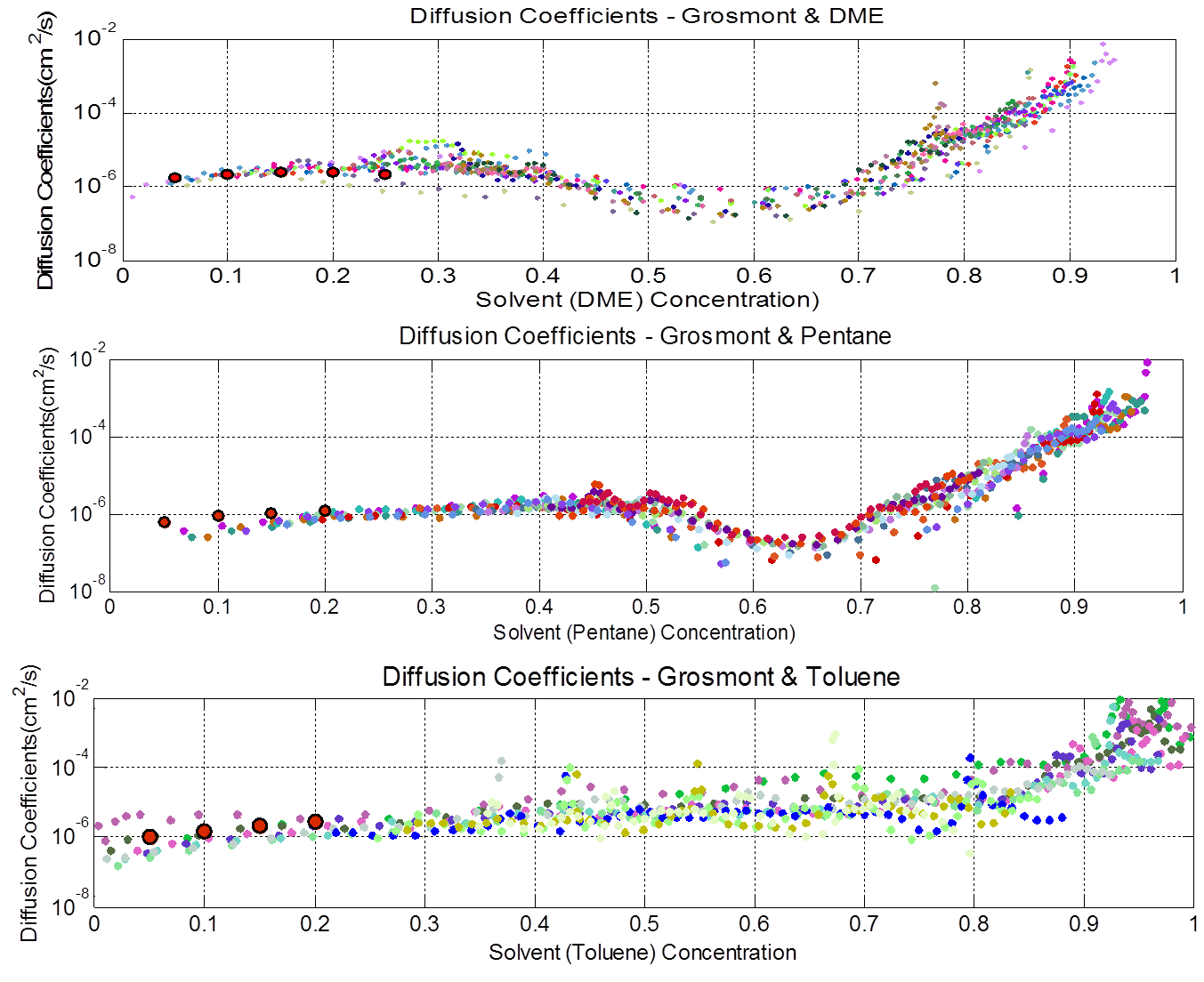
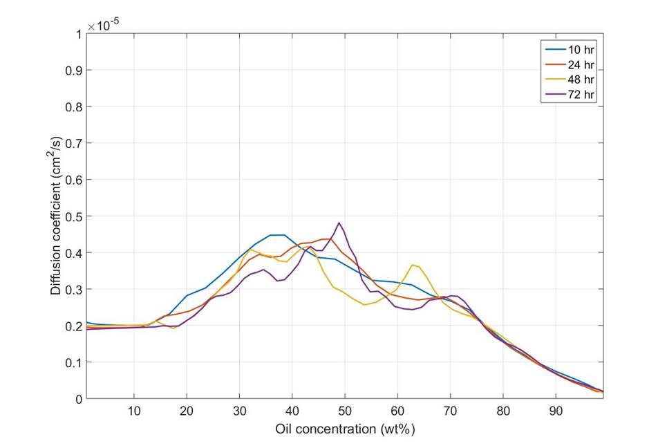
- Diffusion coefficient was obtained from concentration profiles and solving the diffusion equation
- Diffusion coefficient is a strong function of concentration
- PLEASE NOTE THE DIFFERENCE IN SHAPE
- THIS IS A DIRECT RESULT OF THE INTERPRETATION MODEL USED
- Different MODELS ARE TESTED
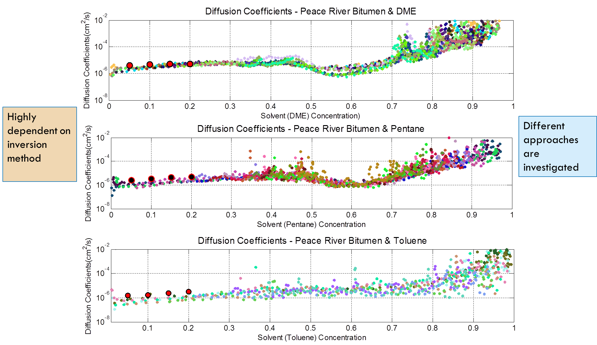
- Diffusion coefficient was obtained from concentration profiles and solving the diffusion equation
- Diffusion coefficient is a strong function of concentration
- PLEASE NOTE THE DIFFERENCE IN SHAPE
- THIS IS A DIRECT RESULT OF THE INTERPRETATION MODEL USED
- Different MODELS ARE TESTED
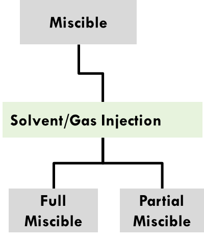
Miscible Displacements
Modelling Process
Solving equations of flow and transport:
- Continuity equatio
∇.(ρu)=0
- Navier-Stokes equation
ρ ∂u/∂t+ρ(u.∇)u=∇.[-pI+μ∇u]+ρg
- Convection-Diffusion equation
∂c/∂t+∇.(-D∇c)+u.∇c=0
Flow Properties
Simulations are being conducted at various flow conditions:
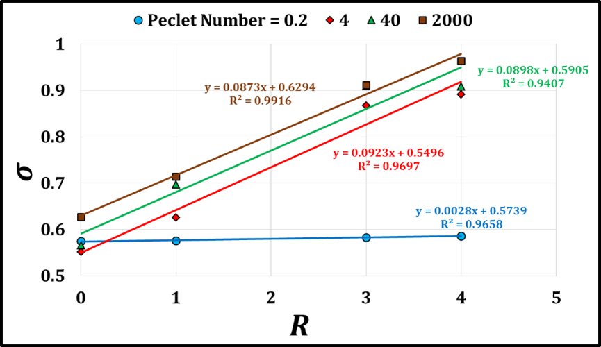
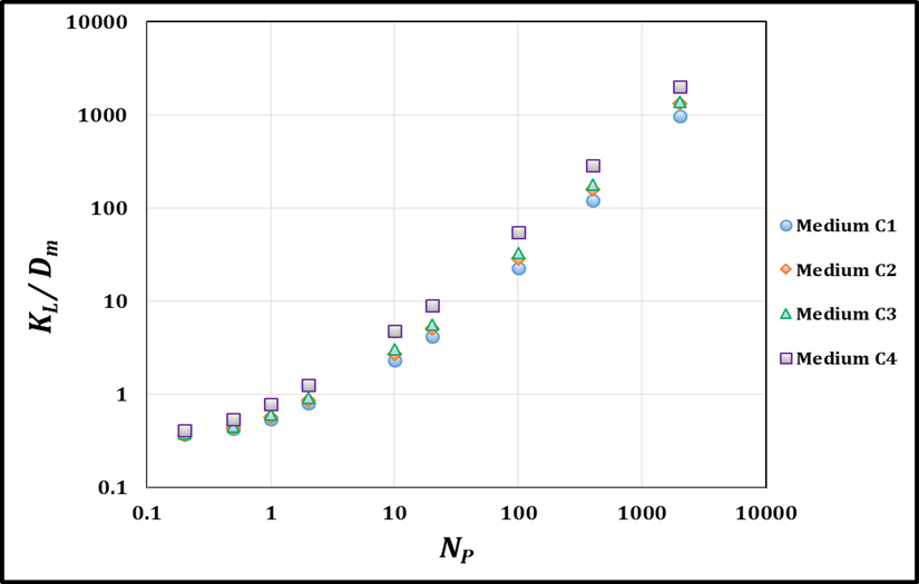
- Wide range of displacement velocity in terms of Peclet number (N_P)
- Various viscosity ratios in terms of log-viscosity ratio (R=ln(μ_displaced/μ_displacing ))
- Incorporation of gravity effects
- Incorporation of concentration dependent diffusion coefficient
- Multicomponent mass transfer
Modelling Outcomes
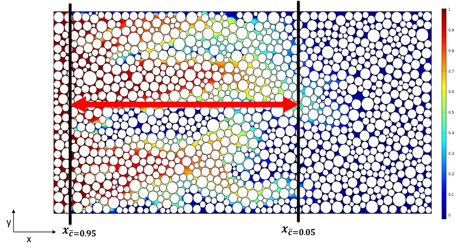
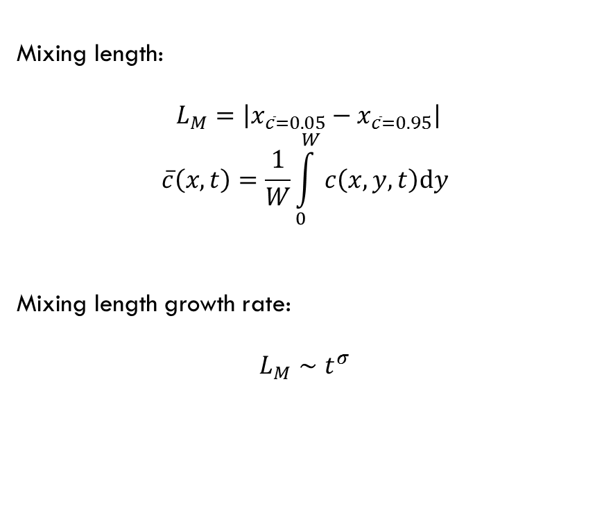
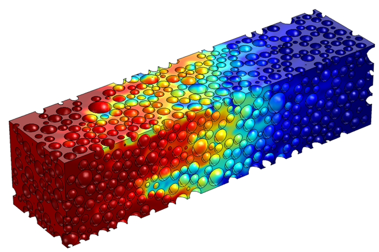
Mixing zone growth rate (σ) at different flow conditions:
Mixing zone length calculation:
- Effect of Peclet number and viscosity ratio
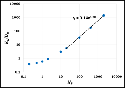
- Dispersion coefficient calculation:
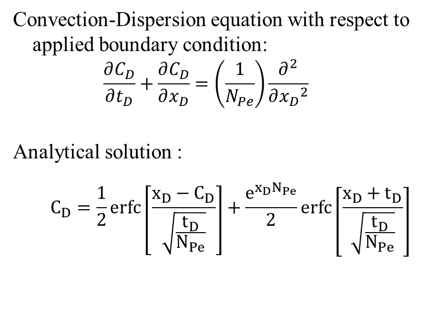
At macro-scale, longitudinal dispersion can be described by a convection-dispersion equation:
∂c/∂t+∇.(-K_L ∇c)+u.∇c=0
K_L in a porous media along the flow direction can be calculated by matching the numerically obtained concentration profile at the outlet with the analytical semi-infinite solution of convection-dispersion equation.
- Effect of Viscosity ratio
Partial Miscibility
- Concentration shock or continual interface renewal at the interface between the undiluted heavy oil and solvent vapour can be one of the reasons for higher production rates than expected
- Low-viscosity diluted heavy oil adjacent to the interface flows away from the interface faster than the fluid diffuses into the heavy oil
- Three forces acting on a drop/slug/film of fluid within a porous medium: Gravity, Interfacial Tension and Viscous Forces
- Gravity must overcome interfacial forces during gravity drainage to cause the fluid to move. Only once the fluid is moving, viscosity come into play
- Solve transport of species in continuous liquid and gas phases and across fluid interfaces (convection-diffusion equation)
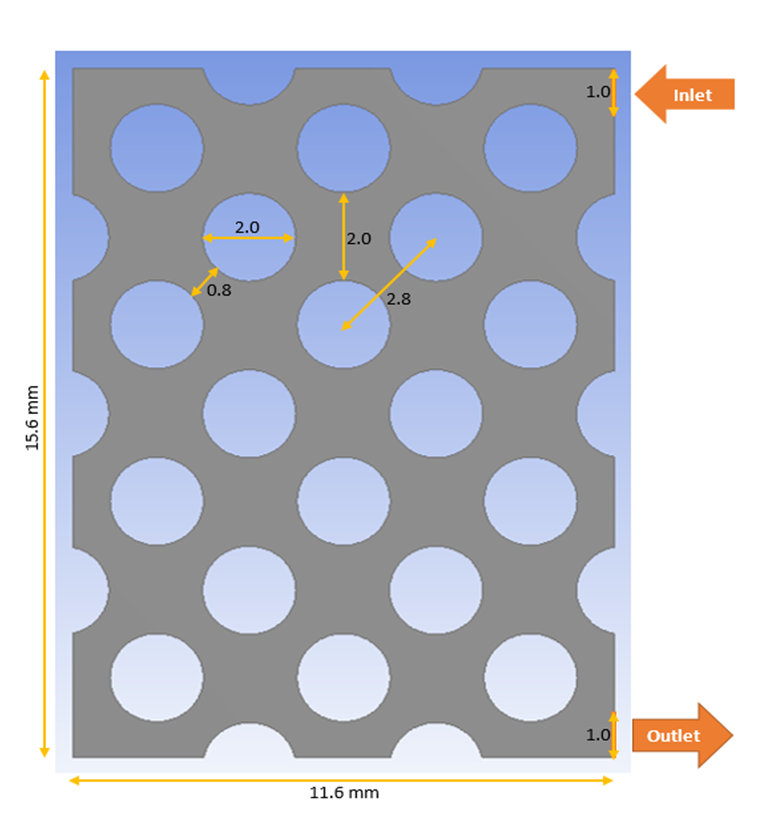
- Based on color function volume-of-fluid (CF-VOF) method
- Each computational cell stores pressure, velocity, phase volume fraction and concentration of species (solvent)
- Viscosity of the heavy oil and solvent mixture was modeled as a function of concentration of diffused solvent in heavy oil
Effect of IFT
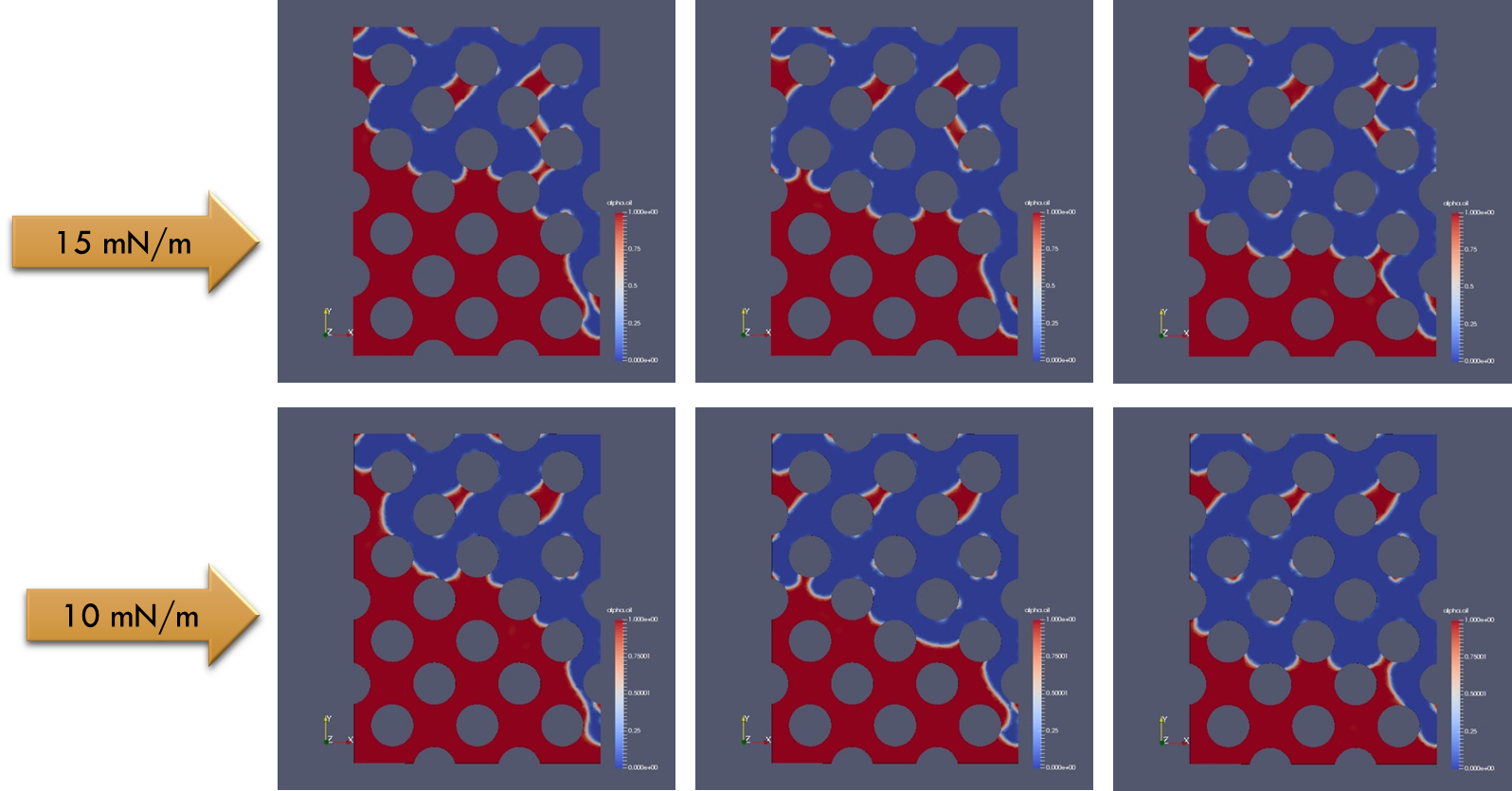
The Case of 0.015mN/m
Phase Change Phenomena
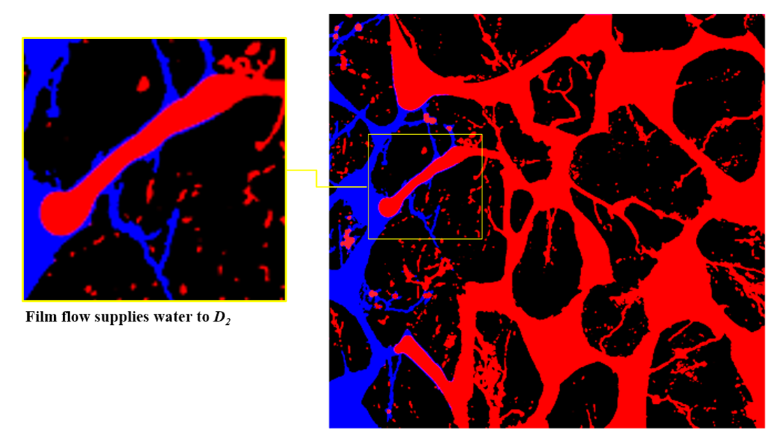
SAGD Modelling at the pore level
Numerous experiments
What is the thickness of condensate?
Phase changes in a steam flood
Mineral Heterogeneity
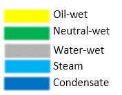
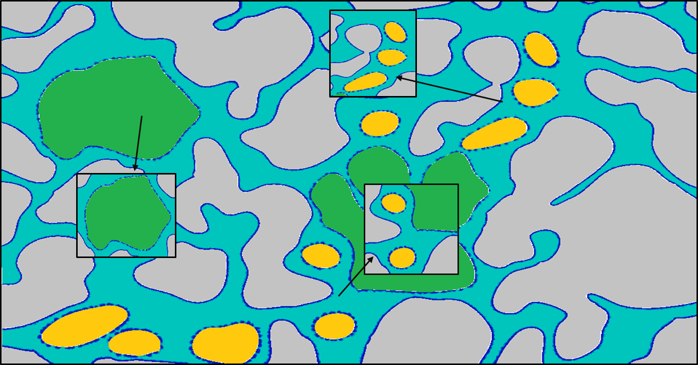
Experiment vs. Modelling; Lab SAGD
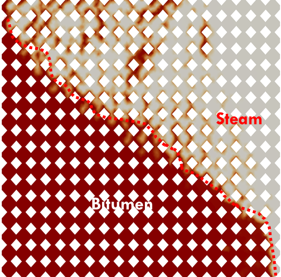
Modelling
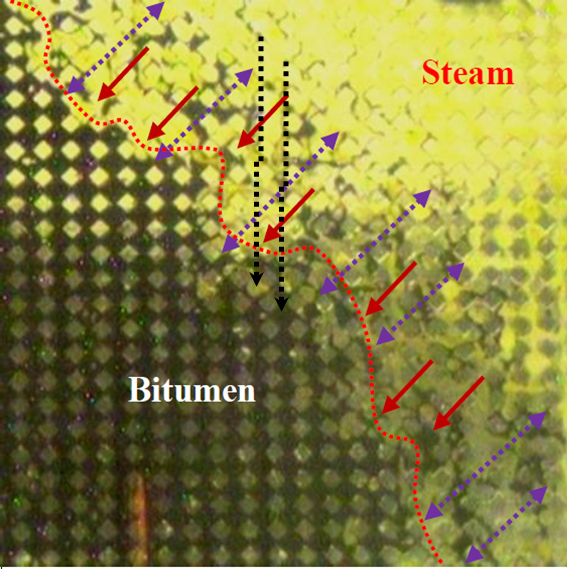
Experiment
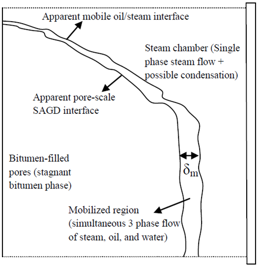
Theory
- Viscosity ratio: 10000 at 25oC
- Density ratio: 1
- Neutral wet
- Saturation Temperature: 373.15K
- Steam Temperature: 403.15K
- Oil Temperature: 298.15K
- IFT: Steam-Water=0.071 Nm-1
- IFT: Oil-Water=0.0341 Nm-1
- IFT: Steam-Oil=0.024 Nm-1

Geometry
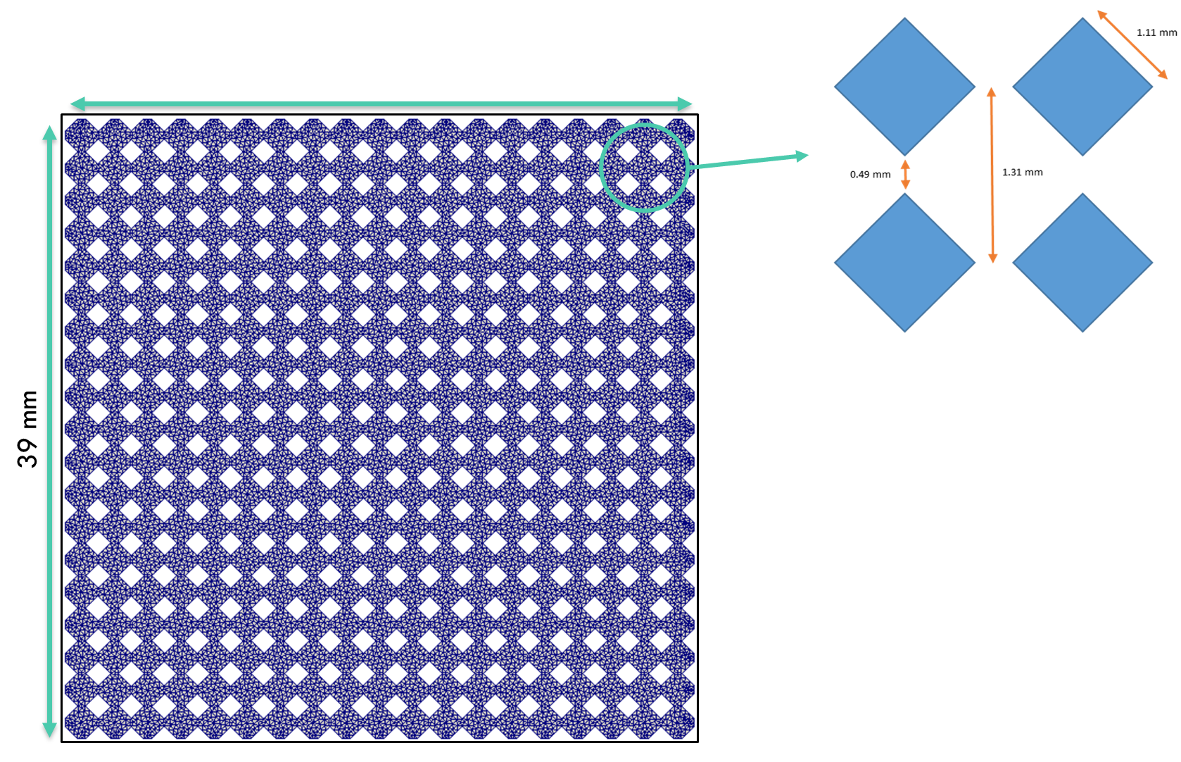
Fluid Properties
Table 5-2: Fluid Properties
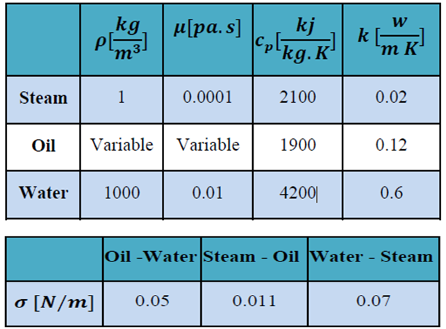
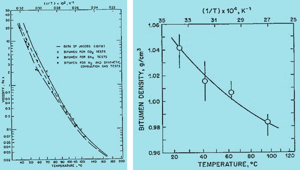
Figure 5-3: (a) Viscosity functionality, (b) Density functionality to temperature
(Svrcek and Mehrotra, 1982)
Boundary and Initial Conditions
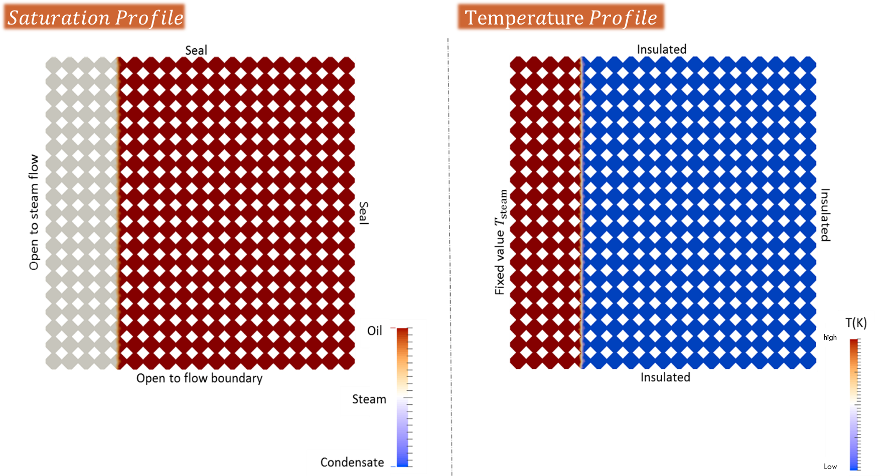
Case Studies

T_sat=100 ℃
Saturation Profiles
Case #1
- Highly efficient heat transfer reduces the accumulation of condensate
Case #3
Dynamic Simulations
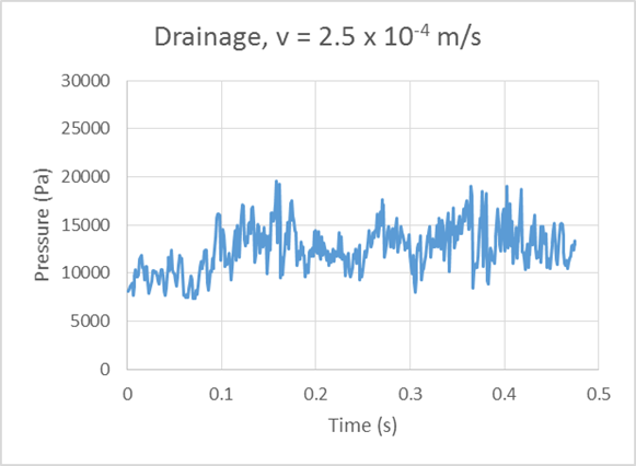
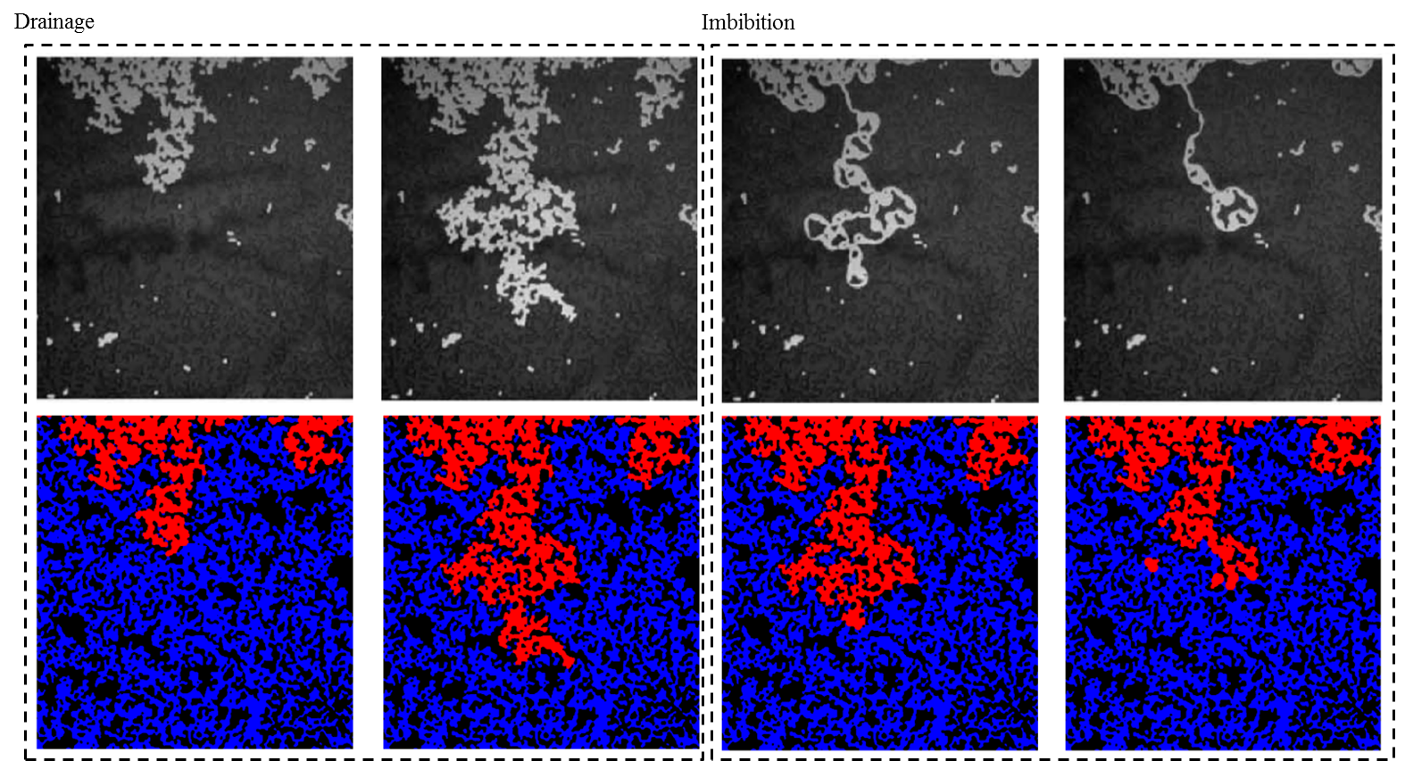
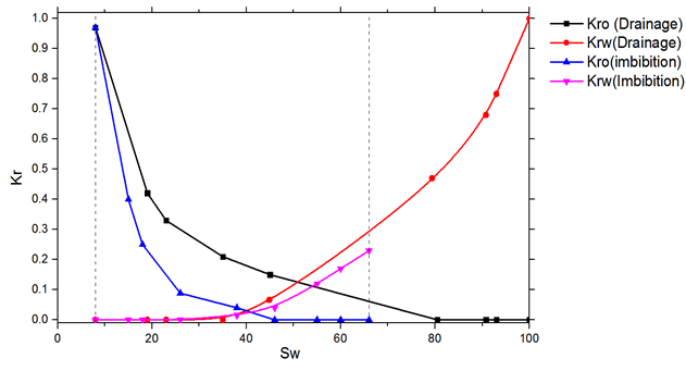
Drainage and Imbibition of viscous oil and water.
Drainage Demonstration – Viscosity Ratio 1:1
Demonstration of Imbibition
T = 140°C and v = 1 x 10⁻³ m/s
- High shear flow
- Local Ca numbers are high enough to result in blob deformation and breakage
- Viscosity Ratio 196
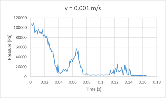
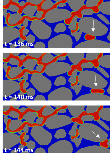
Oil Ganglia Dynamics
- Choke-off is the main mechanism of ganglia break up observed in the runs (120 – 122 ms)
- Oil mobilization happens through successive jumps (122 – 124 ms)
- Once it breaks up, smaller ganglia can get mobilized or stranded, depending on external pressure gradient and local capillary pressure

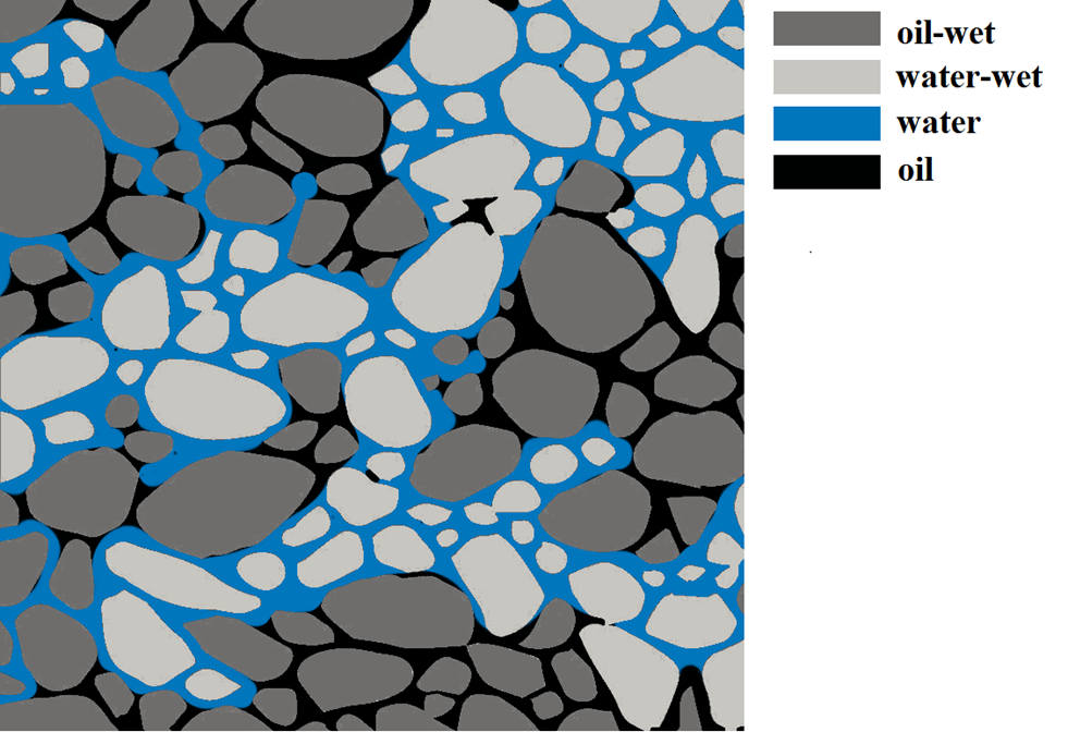
Wettability Heterogeneity
- Fractional-wet
- Dynamic Solver
- Coupled Level Set Volume of Fluid (CLSVOF)
- OpenFoam CFD package
3D VOF-based Simulations
- Unconsolidated sand packing of 1600 grains
- Creation of virtual porous medium with a given particle size distribution
- Numerical simulation of immiscible displacement of primary drainage at different viscosity ratios: In this case the viscosity ratio R=10
Pore-Network Modelling
What can we do when images are not available?
How about when we want quick and dirty results?
How about when we have limited computer capabilities?
Pore Space Simplification
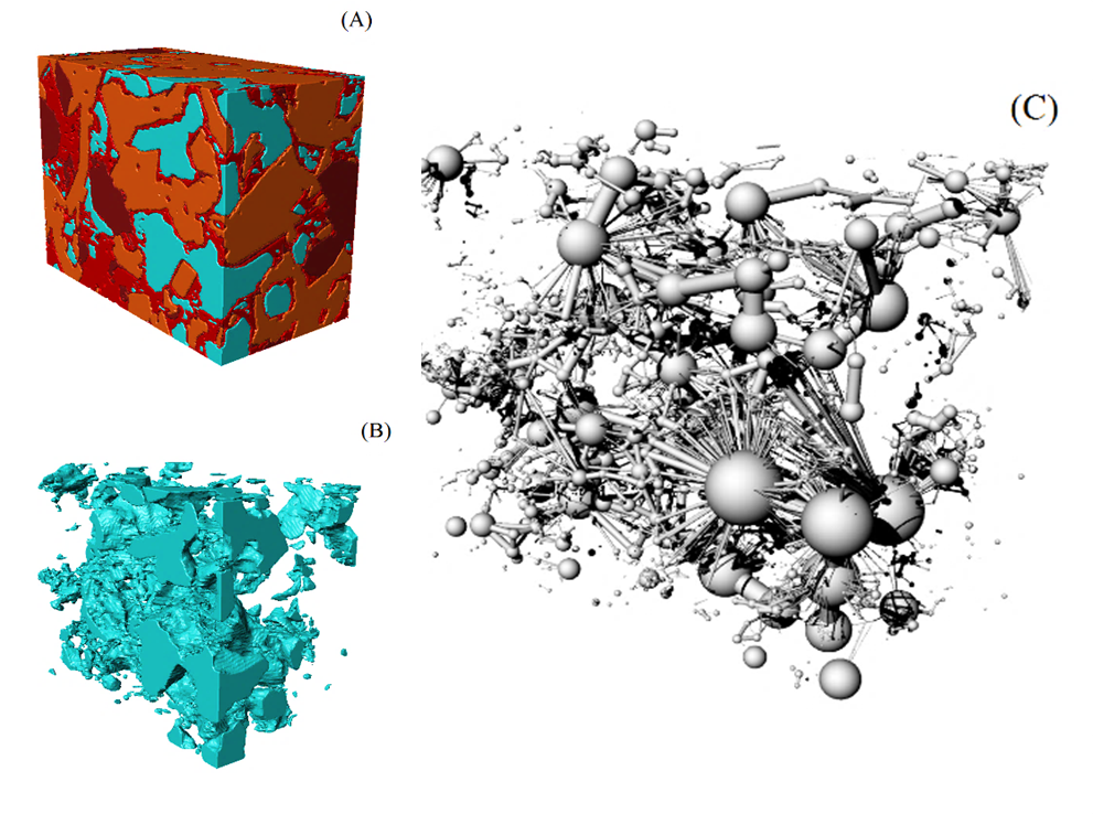
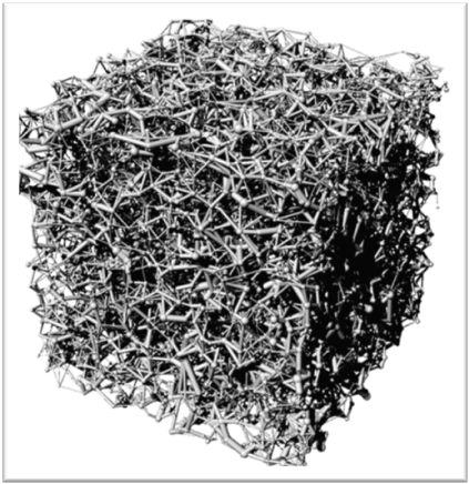
Random Network Model
- Pore bodies interconnected by throats
- Pore Bodies are randomly positioned throughout the space.
Pore Bodies:
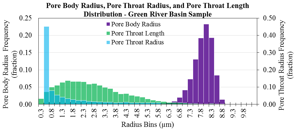
- Size distribution
- Shape factor distribution
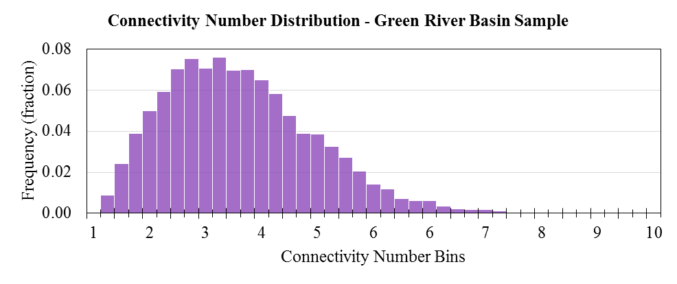
- Connectivity number distribution
Pore Throats:
- Size distribution
- Shape factor distribution
- Length distribution
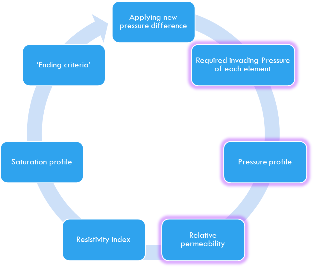
Algorithm
PROCESS:
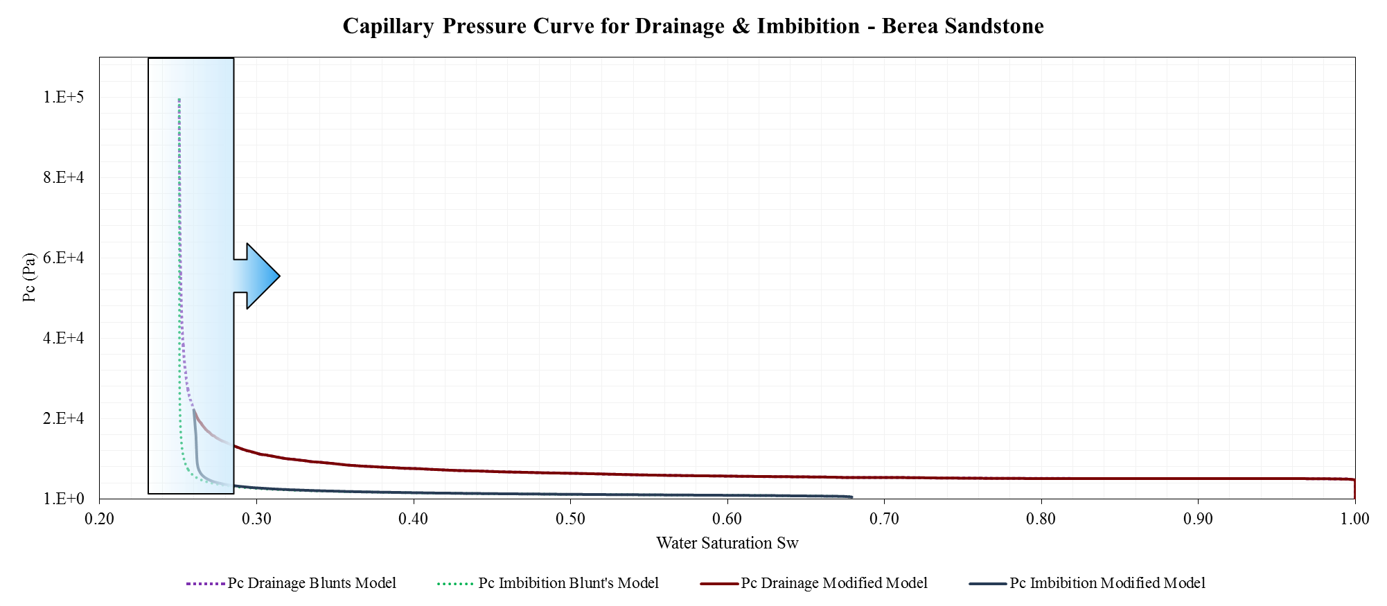
P_c= P_(non-wetting phase)-P_(wetting phase)
Pressure of the non-wetting phase can increase leading to:
- Increase of Pc during drainage
Pressure of the wetting phase can increase leading to:
- Decrease of Pc during imbibition
Berea Sandstone Network Reconstruction
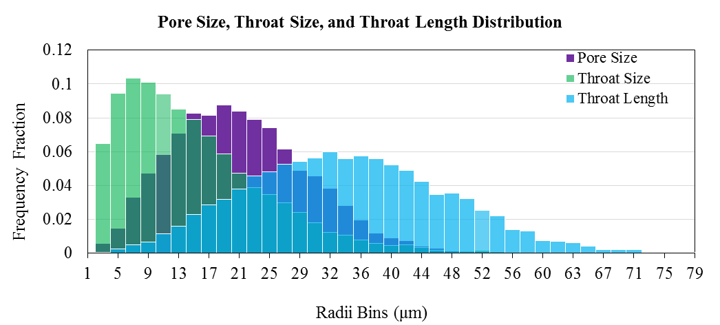
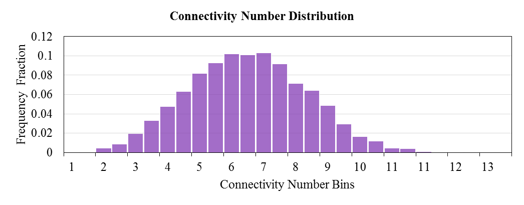
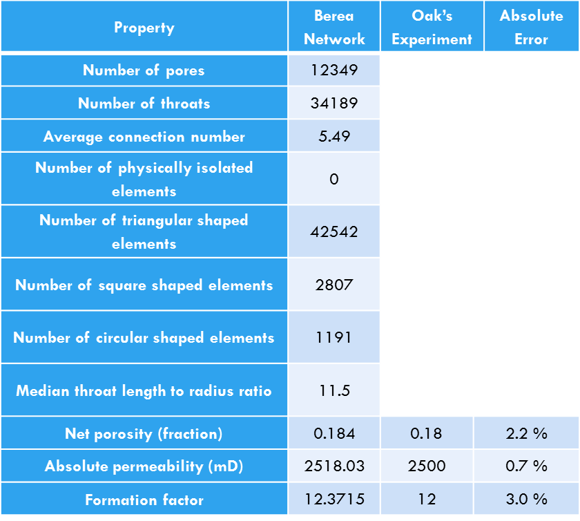
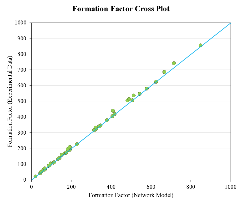
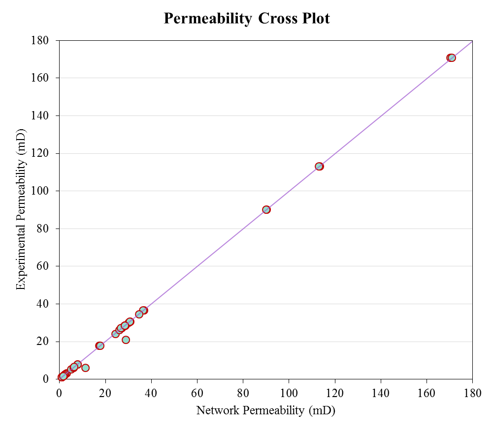
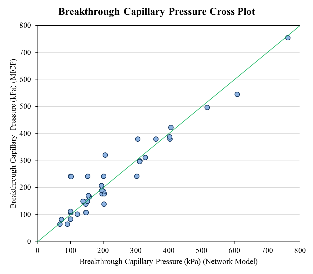
Network Calibration & Validation
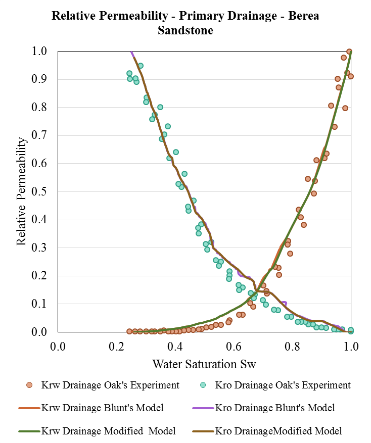
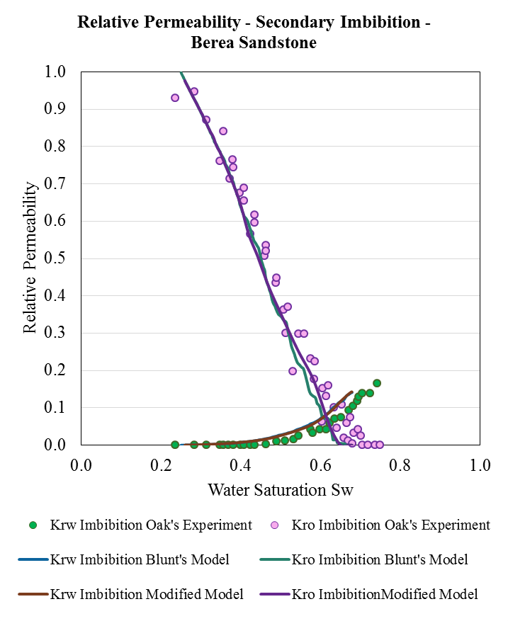
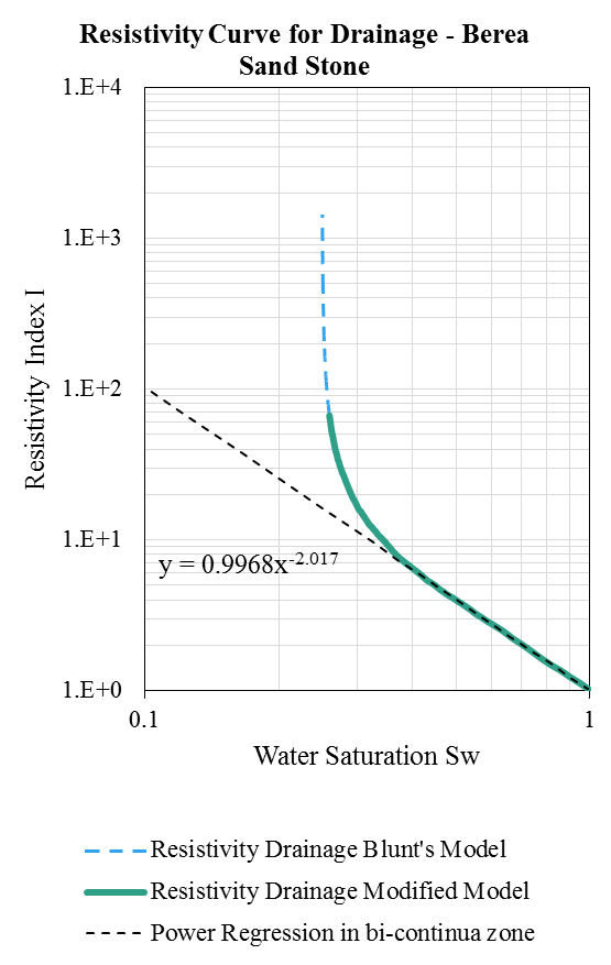
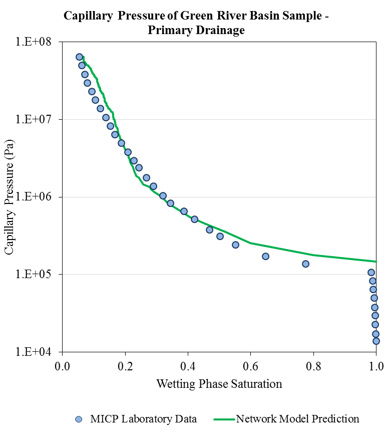
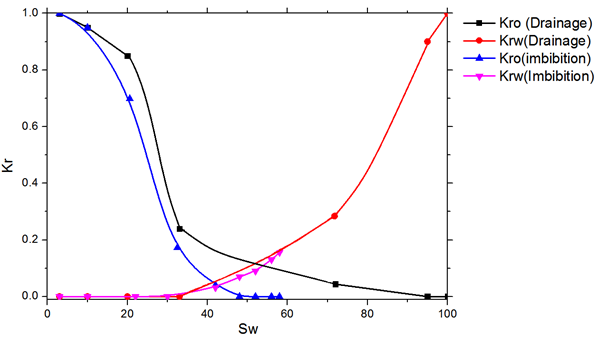
Capillary Pressure Curves
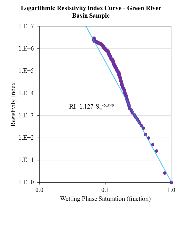
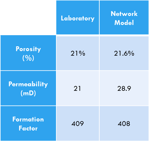
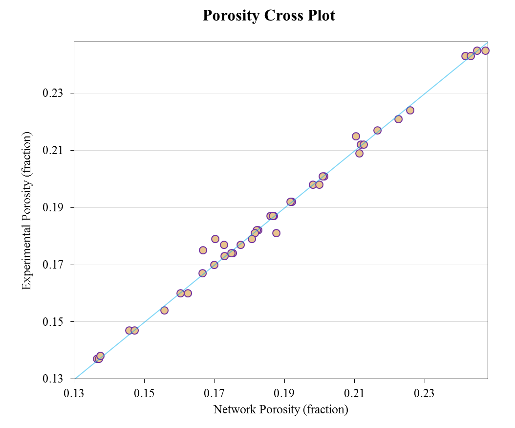
Green River Basin
- Pore throat radius distribution is extracted from mercury porosimetry data.
- Pore throat length distribution is obtained by iteration to match formation factor
- Pore body distribution is obtained by iteration to match porosity and permeability
- Connectivity number distribution is obtained by iteration to match experimental capillary pressure curve
Flow Properties
Pore Morphological Simulations
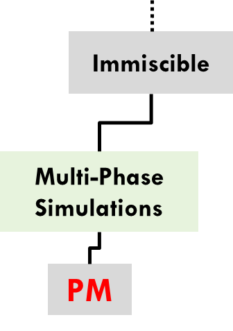
Pore Network Modelling IS FAST BUT TOO SIMPLE
CAN WE APPLY THE RULES OF PNM INTO DIRECT PORE SPACE RECONSTRUCTIONS?
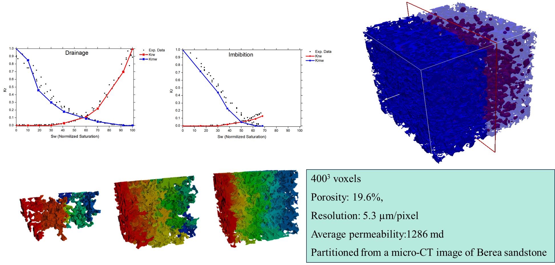
Generate all two-phase properties using the hierarchical rules but the full morphology
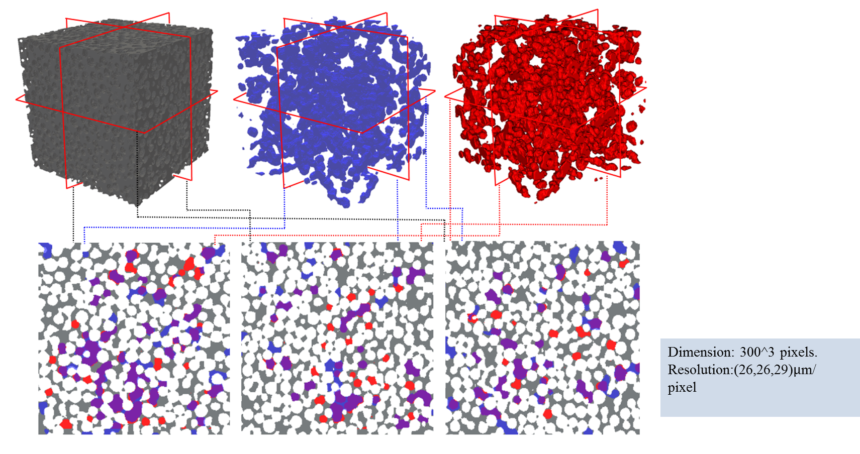
Experimental Validation
Two-Phase Simulations
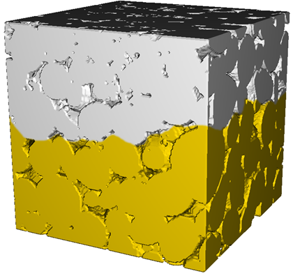
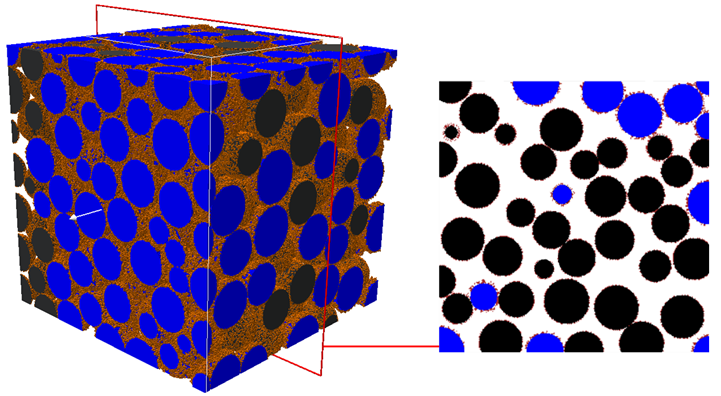
Mixed-wet
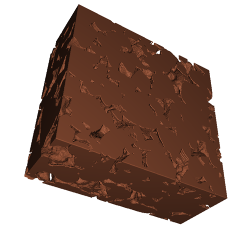
Fractional-Wet
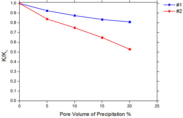
Precipitation
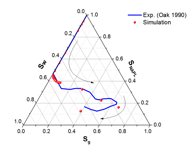
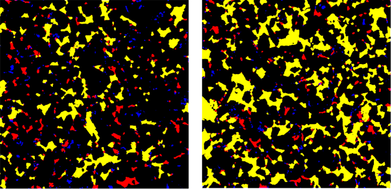
Three -Phase Simulations
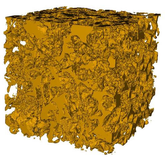
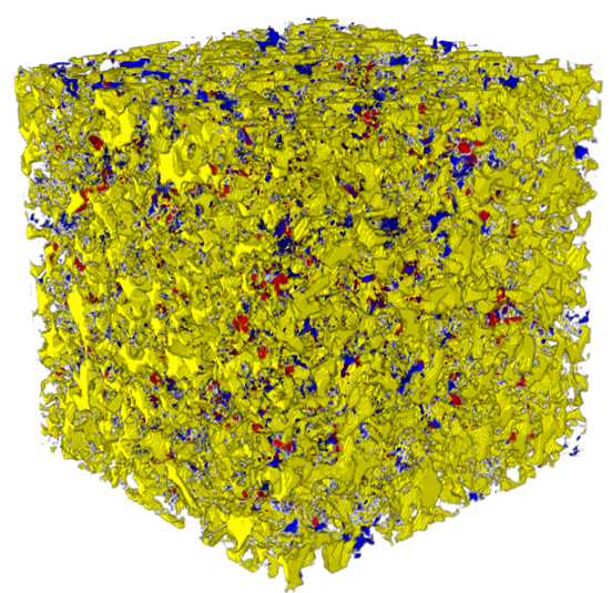
Effective Properties
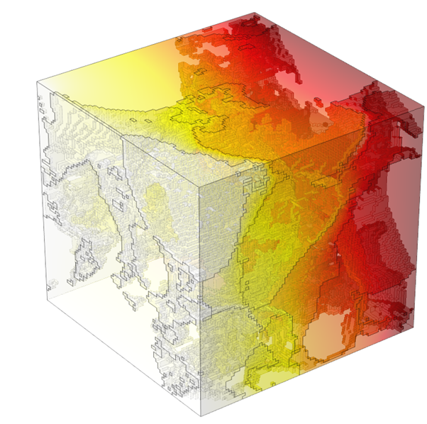
Thermal Conductivity Calculations
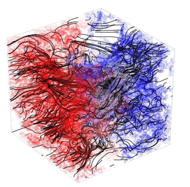
Electrical Resistivity Calculations
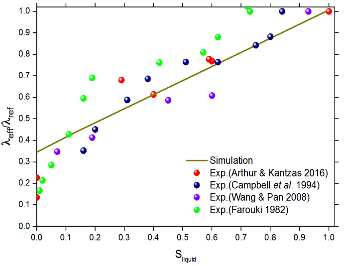
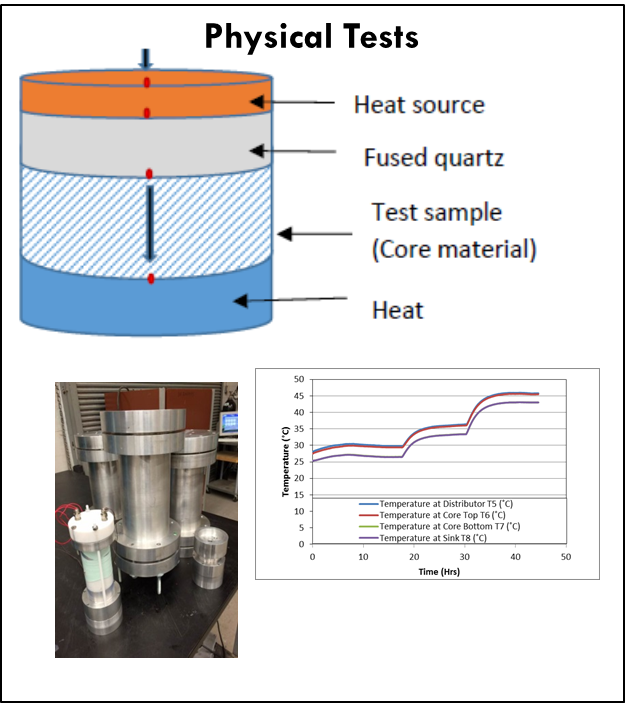
Measurement Technique and Procedure for Thermal Conductivity
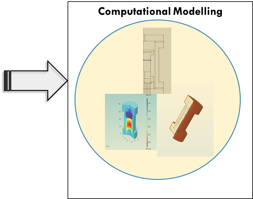
Multi-Scale Simulations
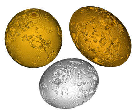
Currently working on combining CFD and PM for complex geometries
Simulation Packages / Software
CFD solvers were implemented in order to:
- Simulate multi-phase isothermal scenarios.
- Simulate thermal processes applying phase change models.
- Simulate mass transfer along the interface during solvent injection.
PNM simulator was adapted in order to:
- Simulate multi-phase capillary dominant displacements.
PM toolbox was developed in order to:
- Simulate multi-phase capillary dominant displacements.
- Predict effective petrophysical, thermal and mechanical properties.
- Simulate multi-sale displacements in a time efficient manner.
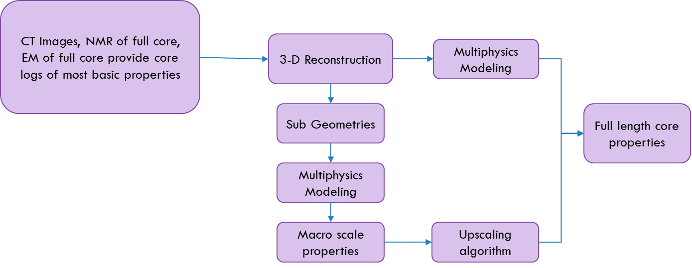
From Micro Scale to Macro Scale
CT Images
Extract images of core and center them.
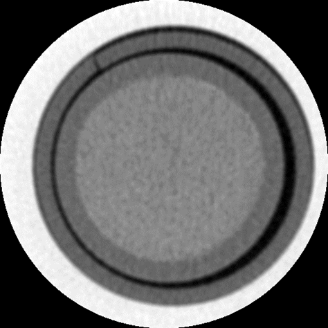
Raw CT Image
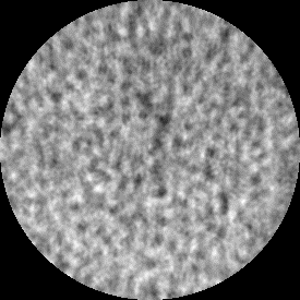
Processed CT Image
3-D Reconstruction of CT
Mask different rock types.
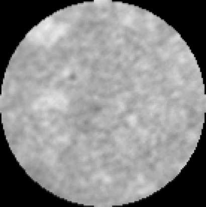
Processed CT Image
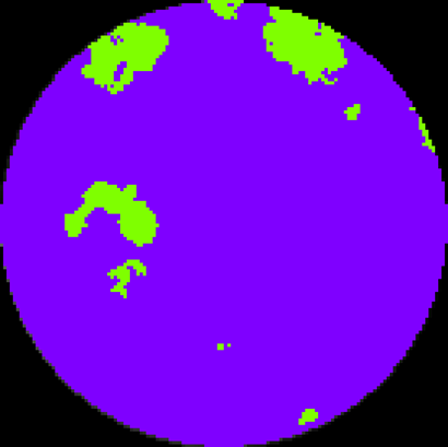
Masked CT Image
3-D Reconstruction of Core
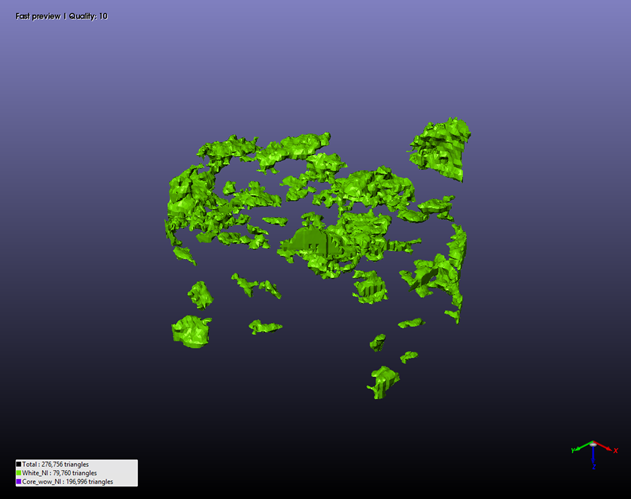
Shaly Sand
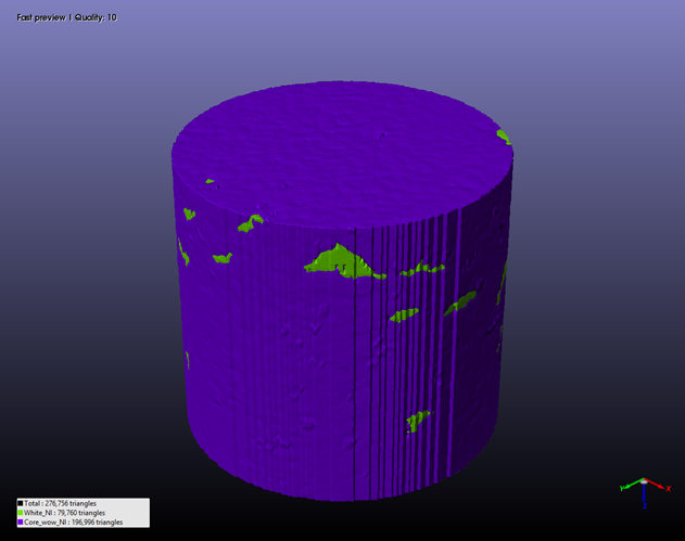
Full Geometry
Multiphysics Modelling of Core and Rock
Apply properties, physics and solve in CFD Software
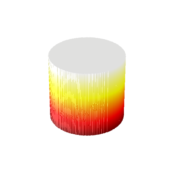
Temperature Profile
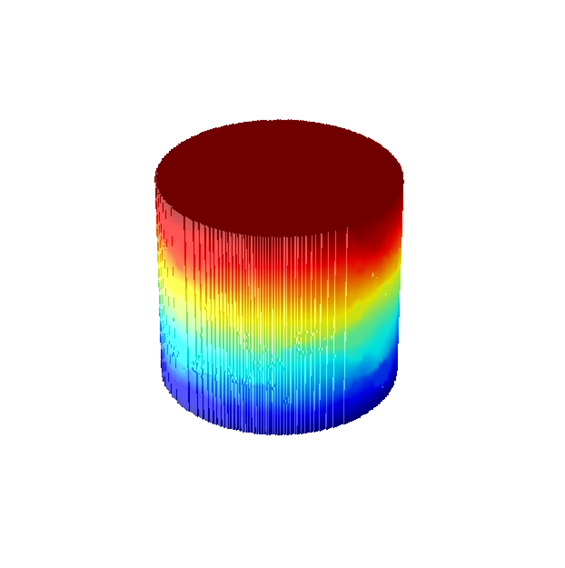
Pressure Profile
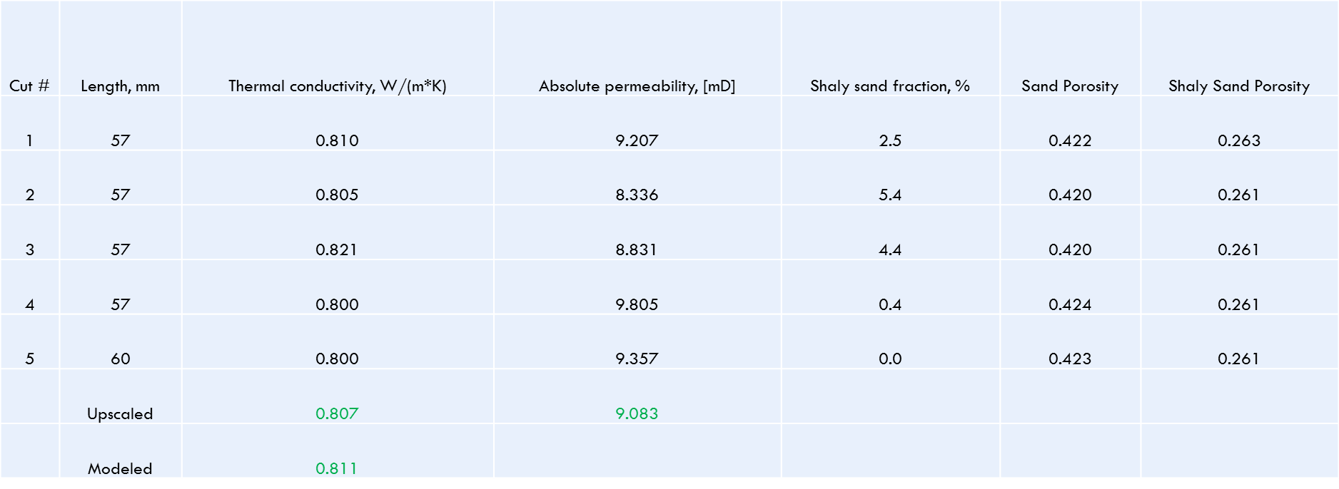
Real Core Example
- Full core decomposed into sub cores
- For each sub core thermal conductivity and permeability was computed
- Using upscaling algorithm properties of full length core were calculated
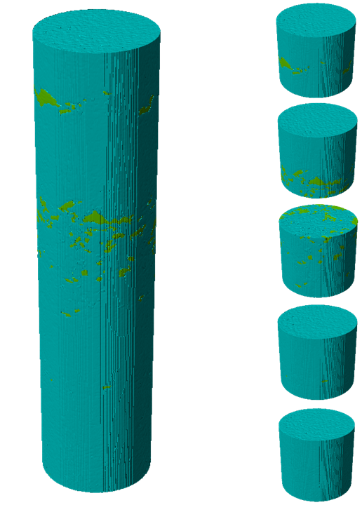
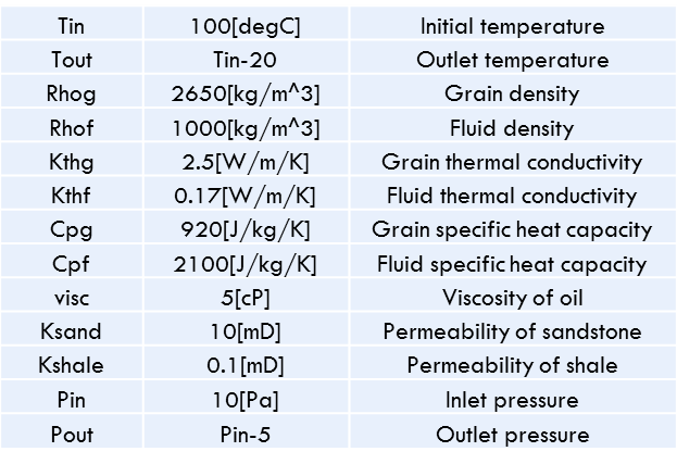
Assumptions and Input Parameters
- Two domains: fluid and rock
- Two rock types: sand and shaly sand
- Geometric mean mixing rule for effective thermal conductivity
- Constant permeability for each rock type
Results
