[1],[2]. The Buckley-Leverett theory [1942] estimates the rate at which an injected water bank moves through a porous medium. The approach uses fractional flow theory and is based on the following assumptions:

• Flow is linear and horizontal
• Water is injected into an oil reservoir
• Oil and water are both incompressible
• Oil and water are immiscible
• Gravity and capillary pressure effects are negligible

In many rocks there is a transition zone between the water and the Oil zones. In the true water zone, the water saturation is essentially 100. In the oil zone, there is usually present connate water, which is essentially immobile. Only water will be produced from a well completed in the true water zone, and only oil will be produced from the true oil zone. In the transition zone both oil and water will be produced, and at each point the fraction of the flowrate that is water will depend on the oil and water saturations at that point.

Frontal advance theory is an application of the law of conservation of mass. Flow through a small volume element () with length ∆x and cross-sectional area “A” can be expressed in terms of total flow rate q_t as:

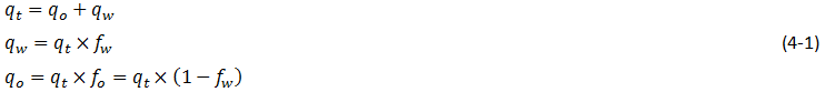
Where q denotes volumetric flow rate at reservoir conditions and the sub-scripts {o,w,t} refer to oil, water, and total rate, respectively and ƒ_w and ƒ_o are fractional flow to water and oil (or water cut and oil cut) respectively:

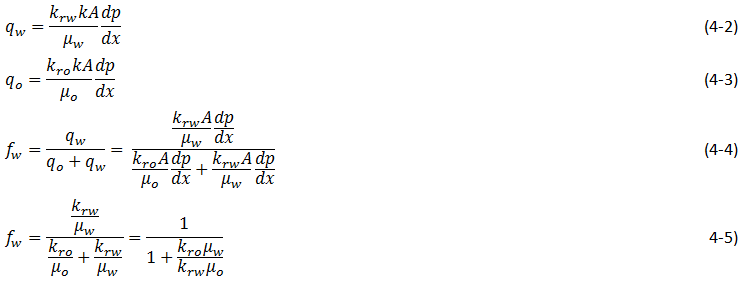
k_o / k_w is a function of saturation. So for constant viscosity ƒ_w is just a function of saturation.

Figure 4‑1 is a plot of the relative permeability ratio, k_o / k_w, versus water saturation. Because of the wide range of k_o / k_w values, the relative permeability ratio is usually plotted on the log scale of semi-log paper. Like many relative permeability ratio curves, the central or main portion of the curve is quite linear. As a straight line on semi-log paper, the relative permeability ratio may be expresses as a function of the water saturation by:

The constants “a” and “b” may be determined from the graph, such as Figure 4‑1, or determined from simultaneous equations from known data of saturation and relative permeability.

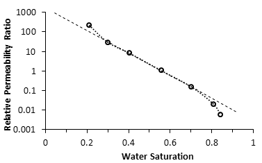
Figure 4-1: Semilog Plot of Relative Permeability Ratio versus Saturation

Substituting eq. (4‑6) into eq. (4‑5) will end with:

If the water fractional flow is plotted versus water saturation, an S-shaped curve will result that is named fractional flow curve.

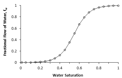
Figure 4-2: Fractional Flow Curve

Assume that the total flow rate is the same at all the medium cross section. Neglect capillary and gravitational forces that may be acting. Let the oil be displaced by water from left to right.

The rate the water enters to the medium element from left hand side (LHS) is:

The rate of water leaving element from the right hand side (RHS) is:

The change in water flow rate across the element is found by performing a mass balance. The movement of mass for an immiscible, incompressible system gives:

Change in Water Flowrate = water entering – water leaving

This is equal to the change in element water content per unit time.

Let S_w is the water saturation of the element at time t. Then if oil is being displaced from the element, at time ( t + Δt ) the water saturation will be ( S_w + ΔS_w ). So water accumulation in the element per unit time is:

Where, φ is porosity. Equating equations (4‑10) and (4‑11) results:

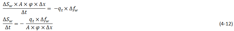
In the limit as ∆t → 0 and ∆x → 0 (for the water phase):

The subscript x on the derivative indicates that this derivative is different for each element.

It is not possible to solve for the general distribution of water saturation S_w( x,t ) in most realistic cases because of the nonlinearity of the problem. For example, water fractional flow is usually a nonlinear function of water saturation. It is therefore necessary to consider a simplified approach to solving Eq. ((4‑13)).

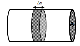
Figure 4-3: Horizontal Bed Containing Oil and Water

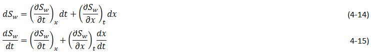
For a given rock, the fraction of flow for water ƒ_w is a function only of the water saturation S_w, as indicated by Eq. (4‑13), assuming constant oil and water viscosities. The water saturation however is a function of both time and position, which may be express as ƒ_w = F( S_w ) and S_w = G( t,x ). Then:

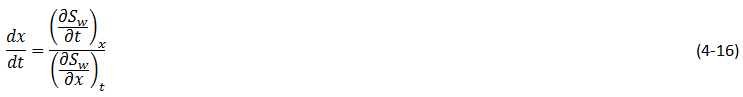
Now, there is interest in determining the rate of advance of a constant saturation plane, or front ( ∂x / ∂t )_Sw , where S_w is constant and dS_w = 0. So from eq. (4‑14):

Substituting eqs (4‑13) and 4‑15) into eq. (4‑16) gives the Buckley-Leverett frontal advance equation:

The derivative is the slope of the fractional flow curve and derivative is the velocity of the moving plane with water saturation S_w. Because the porosity, area, and flowrate are constant and because for any value of S_w, the derivative  is a constant, then the rate dx / dt is constant.

This means that the distance a plane of constant saturation, S_w, advances is proportional to time and to the value of the derivative () at that saturation, or:

Where,

x_Swis the distance traveled by a particular S_w contour

Q_inj is the cumulative water injection at reservoir conditions.

In field units:

Example 4-1

Assume a cubical reservoir under active water drive with oil production of 900bbl/day. The flow could be approximated as a linear flow. The cross sectional area is the product of the width, 1320 ft, and the true formation thickness, 20 ft, so that for a porosity of 0.25, eq. (4‑19) becomes:

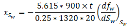
Consider that because we assume the fluids are completely incompressible, so the oil production rate is equal to the total flowrate in the different cross sections of the reservoir.

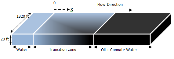
Figure 4-4: Cubic Reservoir Under Active Water Drive

If we let x=0 at the first point of the transition zone, then the distances the various constant water saturation planes will travel in, say, 60, 120, and 240 days are given by:

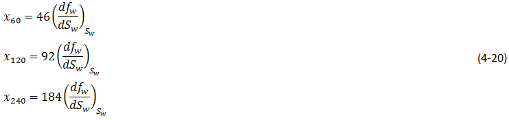
The value of the derivative  may be obtained for any value of water saturation, S_w, by plotting ƒ_w from eq. (4‑7) versus S_w and graphically taking the slopes at various values of S_w. Assume you find a=1222 and b=12 from Figure 4‑1 (intercept = 1222 = ‘a’ and slope of the straight line = 13 = ‘b’) for eq. (4‑7). For example at S_w = 0.4, ƒ_w = 0.129. The slope taken graphically at S_w = 0.4 and ƒ_w = 0.267 is 1.66.

The derivative  may also be obtained mathematically using eq.(4‑7):

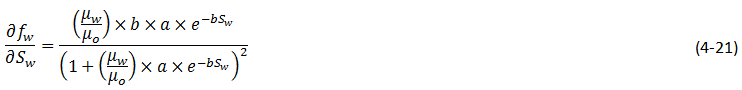
Figure 4‑5 shows the water fractional flow curve and also the derivative  plotted against water saturation from eq. (4‑21). Since Eq. (4‑7) does not hold for the very high and for the quite low water saturation ranges (see Figure 4‑1), some error is introduced below 30% and above 80% water saturation. Since these are in the regions of the lower values of the derivatives, the overall effect on the calculation is small.

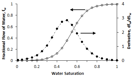
Figure 4-5: Water Fractional Flow and its Derivative

A plot of S_w versus distance using Eq. (4‑20) and typical fractional flow curves leads to the physically impossible situation of multiple values of S_w at a given location. For example Figure 4‑6 shows water saturation distribution according to eqs (4‑20) and (4‑21). For example, at 50% water saturation, the value of the derivative is 2.87; so by eq. (4‑20), at 60 days the 50% water saturation plane will advance a distance of:

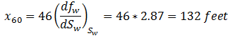
This distance is plotted as shown in Figure 4‑6 along with the other distances that have been calculated using eqs (4‑20) and (4‑21) for other time values and other water saturations. These curves are characteristically double-valued or triple valued. For example, Figure 4‑6 indicates that the water saturation after 240 days at 400 ft is 20, 39, and 69%. The saturation can be only one value at any place and time. What actually occurs is that the intermediate values of the water saturation have the maximum velocity (Figure 4‑5 and eq. (4‑17)), will initially tend to overtake the lower saturations resulting in the formation of a saturation discontinuity or shock front. Because of this discontinuity the mathematical approach of Buckley-Leverett, which assumes that S_w is continuous and differentiable, will be inappropriate to describe the situation at the front itself.

The difficulty is resolved by dropping perpendiculars at point X_ƒ (as flood front position) so that the areas to the right (A) equal the areas to the left (B), as shown in Figure 4‑6. In other words a discontinuity in S_w at a flood front location X_ƒ is needed to make the water saturation distribution single valued and to provide a material balance for displacing fluid.

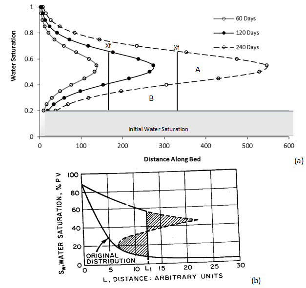
Figure 4-6: (a) Fluid Distribution at 60, 120, 240 days (b) Triple-Valued Saturation Distribution (After Buckley and Leverett, 1942)

A more elegant method of achieving the same result was presented by Welge in 1952. This consists of integrating the saturation distribution over the distance from the injection point to the front, thus obtaining the average water saturation behind the front S_w, as shown in Figure 4‑7[3].

Figure 4-7: Water Saturation Distribution as a Function of Distance, Prior to Breakthrough

The situation depicted is at a fixed time, before water breakthrough, corresponding to an amount of water injection. At this time the maximum water saturation, S_w = 1 – S_or, has moved a distance X1, its velocity being proportional to the slope of the fractional flow curve evaluated for the maximum saturation which, as shown in Figure 4‑5, is small but finite. The flood front saturation S_wƒ is located at position x₂ measured from the injection point. Applying the simple material balance:

So:

Where, Q_inj is cumulative water injection.

Using eq. (4‑18):

At breakthrough time:

Where,

t_bt = Breakthrough time,

q_t = Total injection rate,

L = Medium length

From eq. (4‑24):

Where PVI is the pore volume injected. So:

The average water saturation in the reservoir at the time of breakthrough is given by material balance as:

From eqs (4-26) and (4-27):

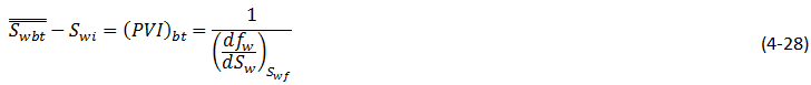
Therefore:

i.e. the slope of the fractional flow curve at conditions of the front is given by eq. 4‑29).

To satisfy eq. (4‑29) the tangent to the fractional flow curve, from the point S_w = S_wc, where ƒ_w = 0, must have a point of tangency with co-ordinates S_w = S_wƒ; ƒ_w = ƒ_wƒ, and extrapolated tangent must intercept the line ƒ_w = 1 at the point (S_w = S_wbt ; ƒ_w = 1). See Figure 4‑8.

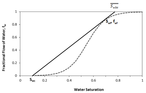
Figure 4-8: Tangent to the Fractional Flow Curve from S_w = S_wc

The use of either of these equations ignores the effect of the capillary pressure gradient, ∂Pc / ∂x.

This simple graphical technique of Welge has much wider application in the field of oil recovery calculations.

As eq. (4‑19) shows the velocity of every saturation front is constant, the graph of saturation location vs. time is set of straight lines starting from the origin. This graph is often plotted in dimensionless form. The equation can be made dimensionless by defining:

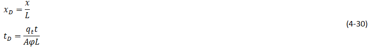
Where

x_D = Normalized distance

t_D = Pore volumes injected

Eq. (4‑19) becomes:

Figure 4‑9 is a graph of dimensionless distance vs. dimensionless time for the movement of water saturation predicted by the frontal advance equation. Saturation S_iw < S_w < S_wƒ travel at the same velocity are located on the flood-front path. The region ahead of flood front has a uniform saturation. Saturations greater than S_wƒ travel at progressively slower velocities as indicated by the decreasing slopes in Figure 4‑9.

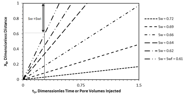
Figure 4-9: x_o vs. t_D for a Linear Waterflooding

Saturation profiles or saturation histories can be constructed by making cross sections through the time/distance graph. A saturation profile is a graph of the locations of all saturations along a cross section of fixed time, as illustrated by the continuous line at t_D = 0.28 in Figure 4‑9. Figure 4‑10 displays the saturation profile at t_D = 0.28 that was obtained from Figure 4‑9.

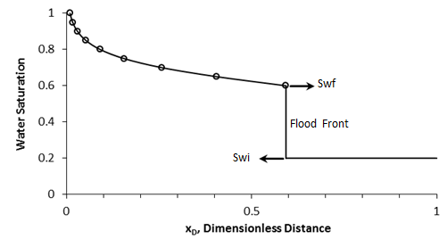
Figure 4-10: Saturation Profile at t_D = 0.28

The saturation history is the graph of saturation vs. time at a particular value of x_D. A plot of water saturation vs. t_D for x_D = 1, shown in Figure 4‑11, illustrates the arrival of water saturations at the end of the linear system.

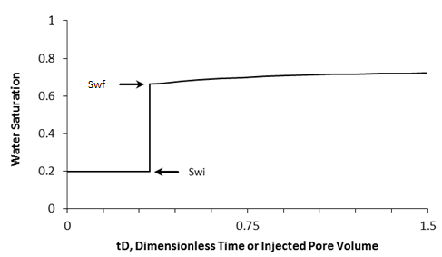
Figure 4-11: Saturation History at x_D = 1, Producing Face of the Medium

Figure 4‑12 represents the initial water and oil distributions in the reservoir unit and also the saturation distributions after 240 days, provided the flood front has not reached the produced face of the cubic reservoir. The area to the right of the flood front in Figure 4‑12 is commonly called the oil bank and the area to the left is sometimes called the flooded or drag zone. The area above the 240-day curve and below the 90% water saturation curve represents oil that may yet be recovered, or dragged out of the high-water saturation portion of the reservoir by flowing large volumes of water through it. The area above the 90% water saturation represents unrecoverable oil since the critical oil saturation is 10%. This presentation of the displacement mechanism has assumed that capillary force is negligible.

Figure 4‑12 also indicates that a well in this reservoir will produce water-free oil until the flood front approaches the well. Thereafter, in a relatively short period, the water cut will rise sharply and be followed by a relatively long period of production at high, and increasingly higher, water cuts. For example, just behind the flood front at 240 days, the water saturation rises from 20% to about 60%-that is, the water cut rises from zero to 66% (see Figure 4‑5). When a producing formation consists of two or more rather definite strata, or stringers, of different permeabilities, the rates of advance in the separate strata will be proportional to their permeabilities, and the overall effect will be a combination of several separate displacements, such as described for a single homogeneous stratum.

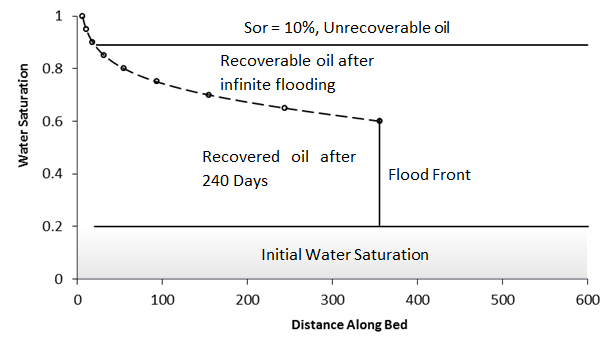
Figure 4-12: Saturation Distribution After 240 Days

References

[1] “Principle of applied reservoir simulation”, John R. Fanchi

[2] “Applied Petroleum Reservoir /engineering”, B.C. Craft, M. Hawkins, 1991

[3] “Fundamentals of Reservoir Engineering”, L.P. Lake, 1978.

Questions?

If you have any questions at all, please feel free to ask PERM!  We are here to help the community.